

254
T. C. Jagadale and S.-W. Chu
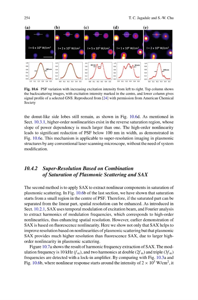
Fig. 10.6 PSF variation with increasing excitation intensity from left to right. Top column shows
the backscattering images, with excitation intensity marked in the centre, and lower column gives
signal profile of a selected GNS. Reproduced from [24] with permission from American Chemical
Society
the donut-like side lobes still remain, as shown in Fig. 10.6d. As mentioned in
Sect. 10.3.1, higher-order nonlinearities exist in the reverse saturation region, whose
slope of power dependency is much larger than one. The high-order nonlinearity
leads to significant reduction of PSF below 100 nm in width, as demonstrated in
Fig. 10.6e. This mechanism is applicable to super-resolution imaging in plasmonic
structures by any conventional laser scanning microscope, without the need of system
modification.
10.4.2 Super-Resolution Based on Combination
of Saturation of Plasmonic Scattering and SAX
The second method is to apply SAX to extract nonlinear components in saturation of
plasmonic scattering. In Fig. 10.6b of the last section, we have shown that saturation
starts from a small region in the centre of PSF. Therefore, if the saturated part can be
separated from the linear part, spatial resolution can be enhanced. As introduced in
Sect. 10.2.1, SAX uses temporal modulation of excitation beam, and Fourier analysis
to extract harmonics of modulation frequencies, which corresponds to high-order
nonlinearities, thus enhancing spatial resolution. However, earlier demonstration of
SAX is based on fluorescence nonlinearity. Here we show not only that SAX helps to
improve resolution based on nonlinearities of plasmonic scattering but that plasmonic
SAX provides much higher resolution than fluorescence SAX, due to larger highorder nonlinearity in plasmonic scattering.
Figure 10.7a shows the result of harmonic frequency extraction of SAX. The modulation frequency is 10 kHz (f m ), and two harmonics at double (2f m ) and triple (3f m )
frequencies are detected with a lock-in amplifier. By comparing with Fig. 10.3a and
Fig. 10.6b, where nonlinear response starts around the intensity of 2 × 10
5 W/cm
2 , it
T. C. Jagadale and S.-W. Chu
Fig. 10.6 PSF variation with increasing excitation intensity from left to right. Top column shows
the backscattering images, with excitation intensity marked in the centre, and lower column gives
signal profile of a selected GNS. Reproduced from [24] with permission from American Chemical
Society
the donut-like side lobes still remain, as shown in Fig. 10.6d. As mentioned in
Sect. 10.3.1, higher-order nonlinearities exist in the reverse saturation region, whose
slope of power dependency is much larger than one. The high-order nonlinearity
leads to significant reduction of PSF below 100 nm in width, as demonstrated in
Fig. 10.6e. This mechanism is applicable to super-resolution imaging in plasmonic
structures by any conventional laser scanning microscope, without the need of system
modification.
10.4.2 Super-Resolution Based on Combination
of Saturation of Plasmonic Scattering and SAX
The second method is to apply SAX to extract nonlinear components in saturation of
plasmonic scattering. In Fig. 10.6b of the last section, we have shown that saturation
starts from a small region in the centre of PSF. Therefore, if the saturated part can be
separated from the linear part, spatial resolution can be enhanced. As introduced in
Sect. 10.2.1, SAX uses temporal modulation of excitation beam, and Fourier analysis
to extract harmonics of modulation frequencies, which corresponds to high-order
nonlinearities, thus enhancing spatial resolution. However, earlier demonstration of
SAX is based on fluorescence nonlinearity. Here we show not only that SAX helps to
improve resolution based on nonlinearities of plasmonic scattering but that plasmonic
SAX provides much higher resolution than fluorescence SAX, due to larger highorder nonlinearity in plasmonic scattering.
Figure 10.7a shows the result of harmonic frequency extraction of SAX. The modulation frequency is 10 kHz (f m ), and two harmonics at double (2f m ) and triple (3f m )
frequencies are detected with a lock-in amplifier. By comparing with Fig. 10.3a and
Fig. 10.6b, where nonlinear response starts around the intensity of 2 × 10
5 W/cm
2 , it