

90
B. Simon and O. Haeberlé
well as the final resolution [71, 72], and can even in some cases lead to misleading
reconstructions [73].
In order to obtain the most accurate reconstructions, and as pointed out by pioneering work in the domain [74, 75], a diffractive approach is to be taken into account,
whose basis is briefly recalled in the next section.
4.3 TDM with Illumination Rotation
In the previous part, digital holographic microscopy was briefly described, highlighting some of its strengths and limitations. In this section, the link between the threedimensional distribution of the sample refractive index and the measurement of its
diffracted field (in phase and amplitude) is recalled, within the scalar approximation
for the sake of simplicity. The interested reader will complete this rapid introduction
by the lecture of classical textbooks on electromagnetism or wave diffraction (for
example [76, 77]), and/or by general introductory reviews of tomographic diffractive
microscopy [78, 79], as well as the seminal papers of the domain [74, 75], and their
extension to high-numerical aperture imaging [80] and take into account the vectorial
nature of the illuminating electromagnetic field [81].
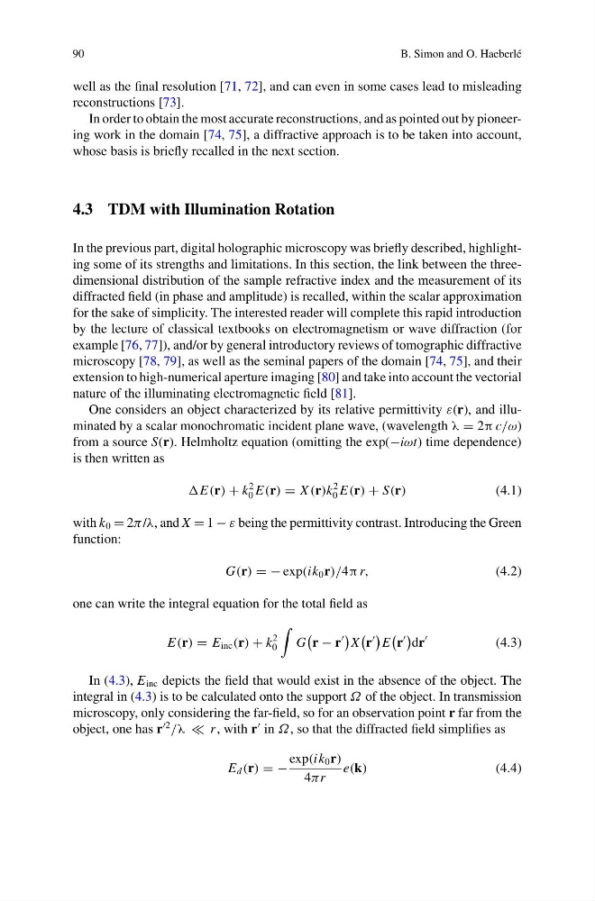
One considers an object characterized by its relative permittivity ε(r), and illuminated by a scalar monochromatic incident plane wave, (wavelength λ = 2π c/ω)
from a source S(r). Helmholtz equation (omitting the exp(−iωt) time dependence)
is then written as
E(r) + k
2
0 E(r) = X (r)k
2
0 E(r) + S(r)
(4.1)
with k 0 = 2π /λ, and X = 1 − ε being the permittivity contrast. Introducing the Green
function:
G(r) = − exp(ik 0 r)/4π r,
(4.2)
one can write the integral equation for the total field as
E(r) = E inc (r) + k
2
0
G
r − r
X
r
E
r
dr
(4.3)
In (4.3), E inc depicts the field that would exist in the absence of the object. The
integral in (4.3) is to be calculated onto the support Ω of the object. In transmission
microscopy, only considering the far-field, so for an observation point r far from the
object, one has r
2
/λ r , with r
in Ω, so that the diffracted field simplifies as
E d (r) = −
exp(ik 0 r)
4πr
e(k)
(4.4)
B. Simon and O. Haeberlé
well as the final resolution [71, 72], and can even in some cases lead to misleading
reconstructions [73].
In order to obtain the most accurate reconstructions, and as pointed out by pioneering work in the domain [74, 75], a diffractive approach is to be taken into account,
whose basis is briefly recalled in the next section.
4.3 TDM with Illumination Rotation
In the previous part, digital holographic microscopy was briefly described, highlighting some of its strengths and limitations. In this section, the link between the threedimensional distribution of the sample refractive index and the measurement of its
diffracted field (in phase and amplitude) is recalled, within the scalar approximation
for the sake of simplicity. The interested reader will complete this rapid introduction
by the lecture of classical textbooks on electromagnetism or wave diffraction (for
example [76, 77]), and/or by general introductory reviews of tomographic diffractive
microscopy [78, 79], as well as the seminal papers of the domain [74, 75], and their
extension to high-numerical aperture imaging [80] and take into account the vectorial
nature of the illuminating electromagnetic field [81].
One considers an object characterized by its relative permittivity ε(r), and illuminated by a scalar monochromatic incident plane wave, (wavelength λ = 2π c/ω)
from a source S(r). Helmholtz equation (omitting the exp(−iωt) time dependence)
is then written as
E(r) + k
2
0 E(r) = X (r)k
2
0 E(r) + S(r)
(4.1)
with k 0 = 2π /λ, and X = 1 − ε being the permittivity contrast. Introducing the Green
function:
G(r) = − exp(ik 0 r)/4π r,
(4.2)
one can write the integral equation for the total field as
E(r) = E inc (r) + k
2
0
G
r − r
X
r
E
r
dr
(4.3)
In (4.3), E inc depicts the field that would exist in the absence of the object. The
integral in (4.3) is to be calculated onto the support Ω of the object. In transmission
microscopy, only considering the far-field, so for an observation point r far from the
object, one has r
2
/λ r , with r
in Ω, so that the diffracted field simplifies as
E d (r) = −
exp(ik 0 r)
4πr
e(k)
(4.4)