

13 Computational Biomechanics of the Brain in the Operating Theatre
335
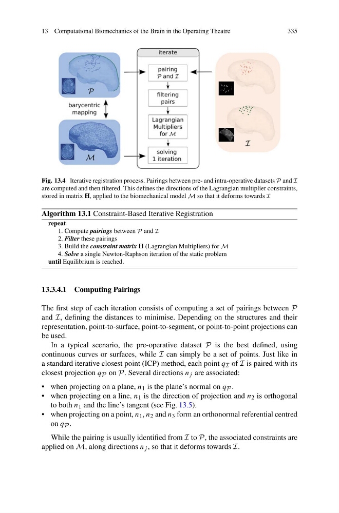
Fig. 13.4 Iterative registration process. Pairings between pre- and intra-operative datasets P and I
are computed and then filtered. This defines the directions of the Lagrangian multiplier constraints,
stored in matrix H, applied to the biomechanical model M so that it deforms towards I
Algorithm 13.1 Constraint-Based Iterative Registration
repeat
1. Compute pairings between P and I
2. Filter these pairings
3. Build the constraint matrix H (Lagrangian Multipliers) for M
4. Solve a single Newton-Raphson iteration of the static problem
until Equilibrium is reached.
13.3.4.1 Computing Pairings
The first step of each iteration consists of computing a set of pairings between P
and I, defining the distances to minimise. Depending on the structures and their
representation, point-to-surface, point-to-segment, or point-to-point projections can
be used.
In a typical scenario, the pre-operative dataset P is the best defined, using
continuous curves or surfaces, while I can simply be a set of points. Just like in
a standard iterative closest point (ICP) method, each point q I of I is paired with its
closest projection q P on P. Several directions n j are associated:
• when projecting on a plane, n 1 is the plane’s normal on q P .
• when projecting on a line, n 1 is the direction of projection and n 2 is orthogonal
to both n 1 and the line’s tangent (see Fig. 13.5).
• when projecting on a point, n 1 , n 2 and n 3 form an orthonormal referential centred
on q P .
While the pairing is usually identified from I to P, the associated constraints are
applied on M, along directions n j , so that it deforms towards I.
335
Fig. 13.4 Iterative registration process. Pairings between pre- and intra-operative datasets P and I
are computed and then filtered. This defines the directions of the Lagrangian multiplier constraints,
stored in matrix H, applied to the biomechanical model M so that it deforms towards I
Algorithm 13.1 Constraint-Based Iterative Registration
repeat
1. Compute pairings between P and I
2. Filter these pairings
3. Build the constraint matrix H (Lagrangian Multipliers) for M
4. Solve a single Newton-Raphson iteration of the static problem
until Equilibrium is reached.
13.3.4.1 Computing Pairings
The first step of each iteration consists of computing a set of pairings between P
and I, defining the distances to minimise. Depending on the structures and their
representation, point-to-surface, point-to-segment, or point-to-point projections can
be used.
In a typical scenario, the pre-operative dataset P is the best defined, using
continuous curves or surfaces, while I can simply be a set of points. Just like in
a standard iterative closest point (ICP) method, each point q I of I is paired with its
closest projection q P on P. Several directions n j are associated:
• when projecting on a plane, n 1 is the plane’s normal on q P .
• when projecting on a line, n 1 is the direction of projection and n 2 is orthogonal
to both n 1 and the line’s tangent (see Fig. 13.5).
• when projecting on a point, n 1 , n 2 and n 3 form an orthonormal referential centred
on q P .
While the pairing is usually identified from I to P, the associated constraints are
applied on M, along directions n j , so that it deforms towards I.