

11 Meshless Algorithms for Computational Biomechanics of the Brain
291
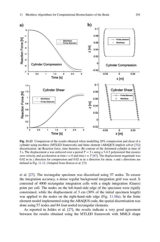
Fig. 11.13 Comparison of the results obtained when modelling 20% compression and shear of a
cylinder using meshless (MTLED framework) and finite element (ABAQUS implicit solver [31])
discretisation. (a) Reaction force, time histories; (b) contour of the deformed cylinder at time of
3 s. The displacement u was enforced over a period T = 3 s using a 3-4-5 polynomial that ensures
zero velocity and acceleration at time t = 0 and time t = T [67]. The displacement magnitude was
0.02 m in z direction for compression and 0.02 m in x direction for shear. x and z directions are
defined in Fig. 11.12. (Adapted from Horton et al. [7])
et al. [27]. The rectangular specimen was discretised using 57 nodes. To ensure
the integration accuracy, a dense regular background integration grid was used. It
consisted of 4000 rectangular integration cells with a single integration (Gauss)
point per cell. The nodes on the left-hand-side edge of the specimen were rigidly
constrained, while the displacement of 3 cm (30% of the initial specimen length)
was applied to the nodes on the right-hand-side edge (Fig. 11.16a). In the finite
element model implemented using the ABAQUS code, the spatial discretisation was
done using 57 nodes and 84 four-noded rectangular elements.
As reported in Joldes et al. [27], the results indicate a very good agreement
between the results obtained using the MTLED framework with MMLS shape
291
Fig. 11.13 Comparison of the results obtained when modelling 20% compression and shear of a
cylinder using meshless (MTLED framework) and finite element (ABAQUS implicit solver [31])
discretisation. (a) Reaction force, time histories; (b) contour of the deformed cylinder at time of
3 s. The displacement u was enforced over a period T = 3 s using a 3-4-5 polynomial that ensures
zero velocity and acceleration at time t = 0 and time t = T [67]. The displacement magnitude was
0.02 m in z direction for compression and 0.02 m in x direction for shear. x and z directions are
defined in Fig. 11.12. (Adapted from Horton et al. [7])
et al. [27]. The rectangular specimen was discretised using 57 nodes. To ensure
the integration accuracy, a dense regular background integration grid was used. It
consisted of 4000 rectangular integration cells with a single integration (Gauss)
point per cell. The nodes on the left-hand-side edge of the specimen were rigidly
constrained, while the displacement of 3 cm (30% of the initial specimen length)
was applied to the nodes on the right-hand-side edge (Fig. 11.16a). In the finite
element model implemented using the ABAQUS code, the spatial discretisation was
done using 57 nodes and 84 four-noded rectangular elements.
As reported in Joldes et al. [27], the results indicate a very good agreement
between the results obtained using the MTLED framework with MMLS shape