

218
V. Kurtcuoglu et al.
L. Lateral Ventricle
Fourth Ventricle
Cisterna Magna
Cerebellar Cistern
Sup. Cerebellar Cistern
Quadrigeminal
Right Ambient Cistern
Left Crural Cistern
Right Crural Cistern
Interpeduncular Cistern
Cortical Subarach. Space
Prepontine Cistern
L. Sylvian Cistern
R. Sylvian Cistern
Premedullary Cistern
R. Cerebellomedullary
L. Cerebellomedullary
Cortical Subarach. Space
Cortical Subarach. Space
L. Trigeminal Cistern
R. Trigeminal Cistern
Third Ventricle
Intervent. Foramina
Left Ambient Cistern
Right Cerebellopontine
R. Vestibular Aqueduct
R. Cochlea
R. Utricle
R. Semicircular Canals
L. Semicircular Canals
Left Cerebellopontine
L. Vestibular Aqueduct
L. Cochlea
L. Utricle
Aqueduct of Sylvius
R. Lateral Ventricle
Pericallosal Cistern
Lamina Terminalis
Carotid Cistern
Chiasmatic Cistern
Interpeduncular Cistern
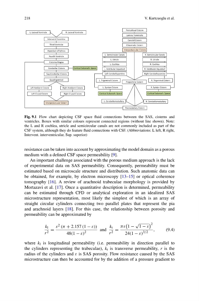
Fig. 9.1 Flow chart depicting CSF space fluid connections between the SAS, cisterns and
ventricles. Boxes with similar colours represent connected regions (without line shown). Note:
the L and R cochlea, utricle and semicircular canals are not commonly included as part of the
CSF system, although they do feature fluid connections with CSF. (Abbreviations: L left, R right,
Intervent. interventricular, Sup. superior)
resistance can be taken into account by approximating the model domain as a porous
medium with a defined CSF space permeability [9].
An important challenge associated with the porous medium approach is the lack
of experimental data on SAS permeability. Consequently, permeability must be
estimated based on microscale structure and distribution. Such anatomic data can
be obtained, for example, by electron microscopy [13–15] or optical coherence
tomography [16]. A review of arachnoid trabeculae morphology is provided by
Mortazavi et al. [17]. Once a quantitative description is determined, permeability
can be estimated through CFD or analytical exploration in an idealized SAS
microstructure representation, most likely the simplest of which is an array of
straight circular cylinders connecting two parallel plates that represent the pia
and arachnoid layers [18]. For this case, the relationship between porosity and
permeability can be approximated by
k l
r 2 =
ε 2 (π + 2.157 (1 − ε))
48(1 − ε)
2
and
k t
r 2 =
πε
1 −
√
1 − ε
2
24(1 − ε)
3/2
,
(9.4)
where k l is longitudinal permeability (i.e. permeability in direction parallel to
the cylinders representing the trabeculae), k t is transverse permeability, r is the
radius of the cylinders and ε is SAS porosity. Flow resistance caused by the SAS
microstructure can then be accounted for by the addition of a pressure gradient to
V. Kurtcuoglu et al.
L. Lateral Ventricle
Fourth Ventricle
Cisterna Magna
Cerebellar Cistern
Sup. Cerebellar Cistern
Quadrigeminal
Right Ambient Cistern
Left Crural Cistern
Right Crural Cistern
Interpeduncular Cistern
Cortical Subarach. Space
Prepontine Cistern
L. Sylvian Cistern
R. Sylvian Cistern
Premedullary Cistern
R. Cerebellomedullary
L. Cerebellomedullary
Cortical Subarach. Space
Cortical Subarach. Space
L. Trigeminal Cistern
R. Trigeminal Cistern
Third Ventricle
Intervent. Foramina
Left Ambient Cistern
Right Cerebellopontine
R. Vestibular Aqueduct
R. Cochlea
R. Utricle
R. Semicircular Canals
L. Semicircular Canals
Left Cerebellopontine
L. Vestibular Aqueduct
L. Cochlea
L. Utricle
Aqueduct of Sylvius
R. Lateral Ventricle
Pericallosal Cistern
Lamina Terminalis
Carotid Cistern
Chiasmatic Cistern
Interpeduncular Cistern
Fig. 9.1 Flow chart depicting CSF space fluid connections between the SAS, cisterns and
ventricles. Boxes with similar colours represent connected regions (without line shown). Note:
the L and R cochlea, utricle and semicircular canals are not commonly included as part of the
CSF system, although they do feature fluid connections with CSF. (Abbreviations: L left, R right,
Intervent. interventricular, Sup. superior)
resistance can be taken into account by approximating the model domain as a porous
medium with a defined CSF space permeability [9].
An important challenge associated with the porous medium approach is the lack
of experimental data on SAS permeability. Consequently, permeability must be
estimated based on microscale structure and distribution. Such anatomic data can
be obtained, for example, by electron microscopy [13–15] or optical coherence
tomography [16]. A review of arachnoid trabeculae morphology is provided by
Mortazavi et al. [17]. Once a quantitative description is determined, permeability
can be estimated through CFD or analytical exploration in an idealized SAS
microstructure representation, most likely the simplest of which is an array of
straight circular cylinders connecting two parallel plates that represent the pia
and arachnoid layers [18]. For this case, the relationship between porosity and
permeability can be approximated by
k l
r 2 =
ε 2 (π + 2.157 (1 − ε))
48(1 − ε)
2
and
k t
r 2 =
πε
1 −
√
1 − ε
2
24(1 − ε)
3/2
,
(9.4)
where k l is longitudinal permeability (i.e. permeability in direction parallel to
the cylinders representing the trabeculae), k t is transverse permeability, r is the
radius of the cylinders and ε is SAS porosity. Flow resistance caused by the SAS
microstructure can then be accounted for by the addition of a pressure gradient to