

132
2. Stochastic frontier analysis (SFA) (Aigner et al. 1977; (Meeusen and Van den
Broek 1977). This method estimates efficiency by using stochastic production
functions.
3. Data Envelopment Analysis (DEA), originally proposed by Charnes et al. (1978)
which measures efficiency relative to a deterministic nonparametric frontier by
using mathematical optimization methods.
Each of these methodologies has its advantages and disadvantages, as can be seen
in the excellent review provided in Lovell (1996). Particularly, we are going to use
DEA estimation method because it requires the minimal level of assumptions
regarding the technology.
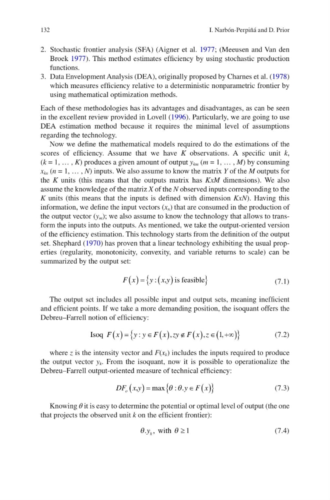
Now we define the mathematical models required to do the estimations of the
scores of efficiency. Assume that we have K observations. A specific unit k,
(k = 1, … , K) produces a given amount of output y km (m = 1, … , M) by consuming
x kn (n = 1, … , N) inputs. We also assume to know the matrix Y of the M outputs for
the K units (this means that the outputs matrix has KxM dimensions). We also
assume the knowledge of the matriz X of the N observed inputs corresponding to the
K units (this means that the inputs is defined with dimension KxN). Having this
information, we define the input vectors (x n ) that are consumed in the production of
the output vector (y m ); we also assume to know the technology that allows to transform the inputs into the outputs. As mentioned, we take the output-oriented version
of the efficiency estimation. This technology starts from the definition of the output
set. Shephard (1970) has proven that a linear technology exhibiting the usual properties (regularity, monotonicity, convexity, and variable returns to scale) can be
summarized by the output set:
F x
y x y
( ) = ( )
{
}
: , is feasible
(7.1)
The output set includes all possible input and output sets, meaning inefficient
and efficient points. If we take a more demanding position, the isoquant offers the
Debreu–Farrell notion of efficiency:
Isoq F x
y y F x zy F x z
( ) =
∈ ( ) ∉ ( ) ∈ +∞
(
)
{
}
:
,
,
,
1
(7.2)
where z is the intensity vector and F(x k ) includes the inputs required to produce
the output vector y k . From the isoquant, now it is possible to operationalize the
Debreu–Farrell output-oriented measure of technical efficiency:
DF x y
y F x
o
,
( )=
∈ ( )
{
}
max : .
θ θ
(7.3)
Knowing θ it is easy to determine the potential or optimal level of output (the one
that projects the observed unit k on the efficient frontier):
θ
θ
. ,
y k with ≥ 1
(7.4)
I. Narbón-Perpiñá and D. Prior
2. Stochastic frontier analysis (SFA) (Aigner et al. 1977; (Meeusen and Van den
Broek 1977). This method estimates efficiency by using stochastic production
functions.
3. Data Envelopment Analysis (DEA), originally proposed by Charnes et al. (1978)
which measures efficiency relative to a deterministic nonparametric frontier by
using mathematical optimization methods.
Each of these methodologies has its advantages and disadvantages, as can be seen
in the excellent review provided in Lovell (1996). Particularly, we are going to use
DEA estimation method because it requires the minimal level of assumptions
regarding the technology.
Now we define the mathematical models required to do the estimations of the
scores of efficiency. Assume that we have K observations. A specific unit k,
(k = 1, … , K) produces a given amount of output y km (m = 1, … , M) by consuming
x kn (n = 1, … , N) inputs. We also assume to know the matrix Y of the M outputs for
the K units (this means that the outputs matrix has KxM dimensions). We also
assume the knowledge of the matriz X of the N observed inputs corresponding to the
K units (this means that the inputs is defined with dimension KxN). Having this
information, we define the input vectors (x n ) that are consumed in the production of
the output vector (y m ); we also assume to know the technology that allows to transform the inputs into the outputs. As mentioned, we take the output-oriented version
of the efficiency estimation. This technology starts from the definition of the output
set. Shephard (1970) has proven that a linear technology exhibiting the usual properties (regularity, monotonicity, convexity, and variable returns to scale) can be
summarized by the output set:
F x
y x y
( ) = ( )
{
}
: , is feasible
(7.1)
The output set includes all possible input and output sets, meaning inefficient
and efficient points. If we take a more demanding position, the isoquant offers the
Debreu–Farrell notion of efficiency:
Isoq F x
y y F x zy F x z
( ) =
∈ ( ) ∉ ( ) ∈ +∞
(
)
{
}
:
,
,
,
1
(7.2)
where z is the intensity vector and F(x k ) includes the inputs required to produce
the output vector y k . From the isoquant, now it is possible to operationalize the
Debreu–Farrell output-oriented measure of technical efficiency:
DF x y
y F x
o
,
( )=
∈ ( )
{
}
max : .
θ θ
(7.3)
Knowing θ it is easy to determine the potential or optimal level of output (the one
that projects the observed unit k on the efficient frontier):
θ
θ
. ,
y k with ≥ 1
(7.4)
I. Narbón-Perpiñá and D. Prior