

154
9 Study of Optical Properties of Biotissues by the Intracavity …
describing the dependence of the real and imaginary parts of the refractive index of
the model structure on the wavelength (dispersion curves and absorption spectra) for
each version of calculations.
The problem includes several stages. At the first stage, the reflectance of a plane
wave from a smoothly irregular layer simulating a given biological structure must
be determined (see Chap. 4).
At the second stage, we must solve the problem of reflection of a Gaussian beam
with an arbitrary cross section from a smoothly irregular layer simulating the given
biological structure. The problem is solved by expanding the fields of counterpropagating waves in plane waves in region 1 of the medium and their reflection from
layer 2 and carrying out inverse transformation followed by the Huygens–Fresnel
integral transformation to obtain the field in the initial reference cross section after
the circumvention of the cavity (see Chap. 4). The constructions at these stages are
auxiliary.
We consider here natural oscillations of a linear resonator loaded with a layer modeling a given biological structure. The constructions are based on solving auxiliary
problems of the first and second stages.
Chapter is based on the results of the [9, 10].
9.2 Integral Equation for Natural Oscillations
of Field in a Resonator
Let a cell with a sample of a biological tissue (tissue section) be located in the vicinity
of the Z axis in domain of the cavity.
Since natural oscillations in ring and linear resonators are retuned in different
ways upon the introduction of inhomogeneities in the cavity, we will consider for
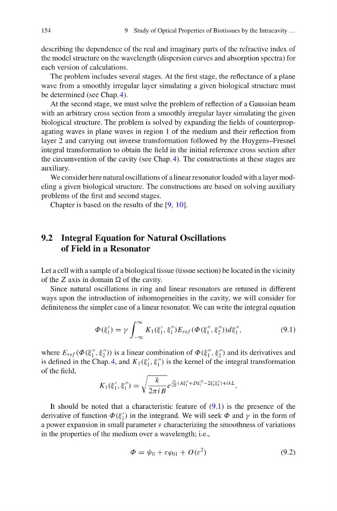
definiteness the simpler case of a linear resonator. We can write the integral equation
Φ(ξ
1 ) = γ
∞
−∞
K 1 (ξ
1 , ξ
1 )E re f (Φ(ξ
1 , ξ
2 ))dξ
1 ,
(9.1)
where E re f (Φ(ξ
1 , ξ
2 )) is a linear combination of Φ(ξ
1 , ξ
2 ) and its derivatives and
is defined in the Chap. 4, and K 1 (ξ
1 , ξ
1 ) is the kernel of the integral transformation
of the field,
K 1 (ξ
1 , ξ
1 ) =
k
2πi B
e
ik
2B (Aξ
1 +Dξ
2
1 −2ξ
1 ξ
1 )+ik L
,
It should be noted that a characteristic feature of (9.1) is the presence of the
derivative of function Φ(ξ
1 ) in the integrand. We will seek Φ and γ in the form of
a power expansion in small parameter ε characterizing the smoothness of variations
in the properties of the medium over a wavelength; i.e.,
Φ = ψ 0 + εϕ 01 + O(ε
2
)
(9.2)
9 Study of Optical Properties of Biotissues by the Intracavity …
describing the dependence of the real and imaginary parts of the refractive index of
the model structure on the wavelength (dispersion curves and absorption spectra) for
each version of calculations.
The problem includes several stages. At the first stage, the reflectance of a plane
wave from a smoothly irregular layer simulating a given biological structure must
be determined (see Chap. 4).
At the second stage, we must solve the problem of reflection of a Gaussian beam
with an arbitrary cross section from a smoothly irregular layer simulating the given
biological structure. The problem is solved by expanding the fields of counterpropagating waves in plane waves in region 1 of the medium and their reflection from
layer 2 and carrying out inverse transformation followed by the Huygens–Fresnel
integral transformation to obtain the field in the initial reference cross section after
the circumvention of the cavity (see Chap. 4). The constructions at these stages are
auxiliary.
We consider here natural oscillations of a linear resonator loaded with a layer modeling a given biological structure. The constructions are based on solving auxiliary
problems of the first and second stages.
Chapter is based on the results of the [9, 10].
9.2 Integral Equation for Natural Oscillations
of Field in a Resonator
Let a cell with a sample of a biological tissue (tissue section) be located in the vicinity
of the Z axis in domain of the cavity.
Since natural oscillations in ring and linear resonators are retuned in different
ways upon the introduction of inhomogeneities in the cavity, we will consider for
definiteness the simpler case of a linear resonator. We can write the integral equation
Φ(ξ
1 ) = γ
∞
−∞
K 1 (ξ
1 , ξ
1 )E re f (Φ(ξ
1 , ξ
2 ))dξ
1 ,
(9.1)
where E re f (Φ(ξ
1 , ξ
2 )) is a linear combination of Φ(ξ
1 , ξ
2 ) and its derivatives and
is defined in the Chap. 4, and K 1 (ξ
1 , ξ
1 ) is the kernel of the integral transformation
of the field,
K 1 (ξ
1 , ξ
1 ) =
k
2πi B
e
ik
2B (Aξ
1 +Dξ
2
1 −2ξ
1 ξ
1 )+ik L
,
It should be noted that a characteristic feature of (9.1) is the presence of the
derivative of function Φ(ξ
1 ) in the integrand. We will seek Φ and γ in the form of
a power expansion in small parameter ε characterizing the smoothness of variations
in the properties of the medium over a wavelength; i.e.,
Φ = ψ 0 + εϕ 01 + O(ε
2
)
(9.2)