

8.3 The Function of Size Distribution or Red Blood Cells
149
modeling blood cells (erythrocytes, leukocytes, platelets, lipoproteins of low density
and lipoproteins of high density). For the numerical determination of f (ρ should be
used Tikhonov regularization method [12].
8.3.1 Tikhonov Regularization Method
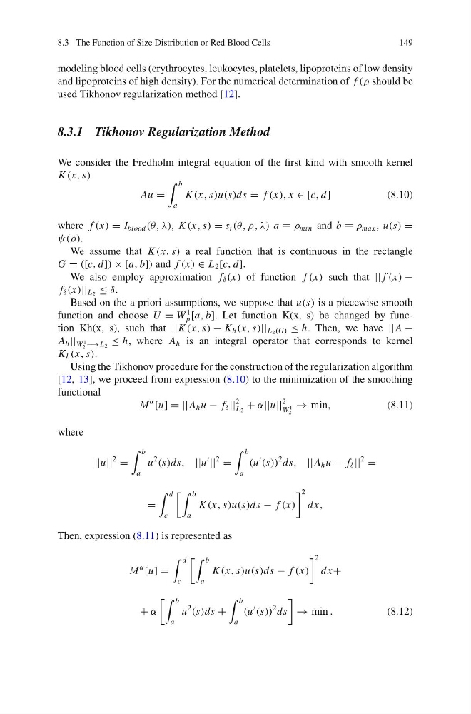
We consider the Fredholm integral equation of the first kind with smooth kernel
K (x, s)
Au =
b
a
K (x, s)u(s)ds = f (x), x ∈ [c, d]
(8.10)
where f (x) = I blood (θ, λ), K (x, s) = s i (θ, ρ, λ) a ≡ ρ min and b ≡ ρ max , u(s) =
ψ(ρ).
We assume that K (x, s) a real function that is continuous in the rectangle
G = ([c, d]) × [a, b]) and f (x) ∈ L 2 [c, d].
We also employ approximation f δ (x) of function f (x) such that || f (x) −
f δ (x)|| L 2 ≤ δ.
Based on the a priori assumptions, we suppose that u(s) is a piecewise smooth
function and choose U = W
1
p [a, b]. Let function K(x, s) be changed by function Kh(x, s), such that ||K (x, s) − K h (x, s)|| L 2 (G) ≤ h. Then, we have ||A −
A h || W
1
2 −→L 2 ≤ h, where A h is an integral operator that corresponds to kernel
K h (x, s).
Using the Tikhonov procedure for the construction of the regularization algorithm
[12, 13], we proceed from expression (8.10) to the minimization of the smoothing
functional
M
α
[u] = ||A h u − f δ ||
2
L 2
+ α||u||
2
W
1
2
→ min,
(8.11)
where
||u||
2
=
b
a
u
2
(s)ds, ||u
||
2
=
b
a
(u
(s))
2 ds, ||A h u − f δ ||
2
=
=
d
c
b
a
K (x, s)u(s)ds − f (x)
2
dx,
Then, expression (8.11) is represented as
M
α
[u] =
d
c
b
a
K (x, s)u(s)ds − f (x)
2
dx+
+ α
b
a
u
2
(s)ds +
b
a
(u
(s))
2 ds
→ min .
(8.12)
149
modeling blood cells (erythrocytes, leukocytes, platelets, lipoproteins of low density
and lipoproteins of high density). For the numerical determination of f (ρ should be
used Tikhonov regularization method [12].
8.3.1 Tikhonov Regularization Method
We consider the Fredholm integral equation of the first kind with smooth kernel
K (x, s)
Au =
b
a
K (x, s)u(s)ds = f (x), x ∈ [c, d]
(8.10)
where f (x) = I blood (θ, λ), K (x, s) = s i (θ, ρ, λ) a ≡ ρ min and b ≡ ρ max , u(s) =
ψ(ρ).
We assume that K (x, s) a real function that is continuous in the rectangle
G = ([c, d]) × [a, b]) and f (x) ∈ L 2 [c, d].
We also employ approximation f δ (x) of function f (x) such that || f (x) −
f δ (x)|| L 2 ≤ δ.
Based on the a priori assumptions, we suppose that u(s) is a piecewise smooth
function and choose U = W
1
p [a, b]. Let function K(x, s) be changed by function Kh(x, s), such that ||K (x, s) − K h (x, s)|| L 2 (G) ≤ h. Then, we have ||A −
A h || W
1
2 −→L 2 ≤ h, where A h is an integral operator that corresponds to kernel
K h (x, s).
Using the Tikhonov procedure for the construction of the regularization algorithm
[12, 13], we proceed from expression (8.10) to the minimization of the smoothing
functional
M
α
[u] = ||A h u − f δ ||
2
L 2
+ α||u||
2
W
1
2
→ min,
(8.11)
where
||u||
2
=
b
a
u
2
(s)ds, ||u
||
2
=
b
a
(u
(s))
2 ds, ||A h u − f δ ||
2
=
=
d
c
b
a
K (x, s)u(s)ds − f (x)
2
dx,
Then, expression (8.11) is represented as
M
α
[u] =
d
c
b
a
K (x, s)u(s)ds − f (x)
2
dx+
+ α
b
a
u
2
(s)ds +
b
a
(u
(s))
2 ds
→ min .
(8.12)