

5 EEG Source Imaging and Multimodal Neuroimaging
87
V (r )
i
g
r i , r di p i , e d i
d i
(5.12)
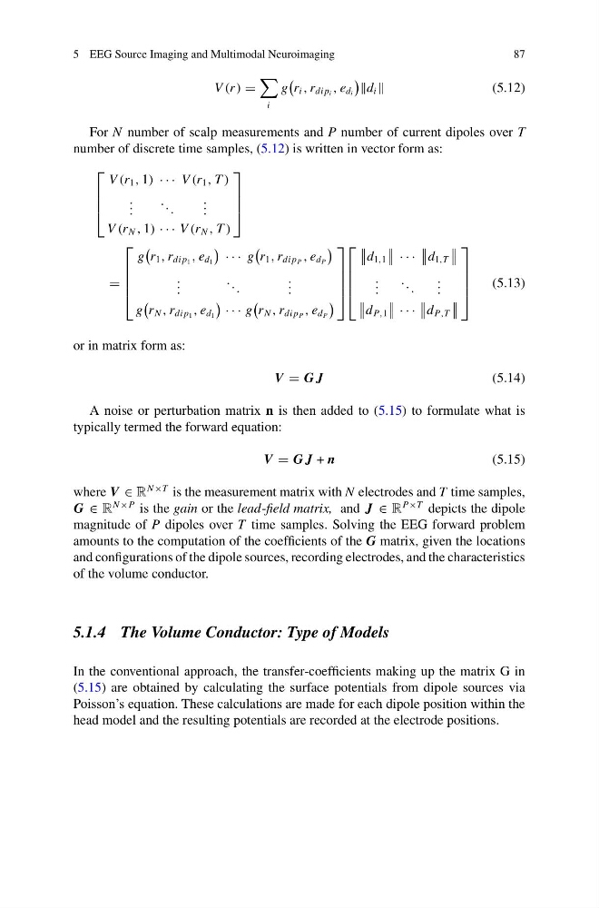
For N number of scalp measurements and P number of current dipoles over T
number of discrete time samples, (5.12) is written in vector form as:
⎡
⎢
⎢
⎣
V (r 1 , 1) · · · V (r 1 , T )
. . .
. . .
. . .
V (r N , 1) · · · V (r N , T )
⎤
⎥
⎥
⎦
⎡
⎢
⎢
⎢
⎣
g
r 1 , r di p 1 , e d 1
· · · g
r 1 , r di p P , e d P
. . .
. . .
. . .
g
r N , r di p 1 , e d 1
· · · g
r N , r di p P , e d P
⎤
⎥
⎥
⎥
⎦
⎡
⎢
⎢
⎢
⎣
d 1,1
· · ·
d 1,T
. . .
. . .
. . .
d P,1
· · ·
d P,T
⎤
⎥
⎥
⎥
⎦
(5.13)
or in matrix form as:
V G J
(5.14)
A noise or perturbation matrix n is then added to (5.15) to formulate what is
typically termed the forward equation:
V G J + n
(5.15)
where V ∈ R
N ×T is the measurement matrix with N electrodes and T time samples,
G ∈ R
N ×P is the gain or the lead-field matrix, and J ∈ R
P×T depicts the dipole
magnitude of P dipoles over T time samples. Solving the EEG forward problem
amounts to the computation of the coefficients of the G matrix, given the locations
and configurations of the dipole sources, recording electrodes, and the characteristics
of the volume conductor.
5.1.4 The Volume Conductor: Type of Models
In the conventional approach, the transfer-coefficients making up the matrix G in
(5.15) are obtained by calculating the surface potentials from dipole sources via
Poisson’s equation. These calculations are made for each dipole position within the
head model and the resulting potentials are recorded at the electrode positions.
87
V (r )
i
g
r i , r di p i , e d i
d i
(5.12)
For N number of scalp measurements and P number of current dipoles over T
number of discrete time samples, (5.12) is written in vector form as:
⎡
⎢
⎢
⎣
V (r 1 , 1) · · · V (r 1 , T )
. . .
. . .
. . .
V (r N , 1) · · · V (r N , T )
⎤
⎥
⎥
⎦
⎡
⎢
⎢
⎢
⎣
g
r 1 , r di p 1 , e d 1
· · · g
r 1 , r di p P , e d P
. . .
. . .
. . .
g
r N , r di p 1 , e d 1
· · · g
r N , r di p P , e d P
⎤
⎥
⎥
⎥
⎦
⎡
⎢
⎢
⎢
⎣
d 1,1
· · ·
d 1,T
. . .
. . .
. . .
d P,1
· · ·
d P,T
⎤
⎥
⎥
⎥
⎦
(5.13)
or in matrix form as:
V G J
(5.14)
A noise or perturbation matrix n is then added to (5.15) to formulate what is
typically termed the forward equation:
V G J + n
(5.15)
where V ∈ R
N ×T is the measurement matrix with N electrodes and T time samples,
G ∈ R
N ×P is the gain or the lead-field matrix, and J ∈ R
P×T depicts the dipole
magnitude of P dipoles over T time samples. Solving the EEG forward problem
amounts to the computation of the coefficients of the G matrix, given the locations
and configurations of the dipole sources, recording electrodes, and the characteristics
of the volume conductor.
5.1.4 The Volume Conductor: Type of Models
In the conventional approach, the transfer-coefficients making up the matrix G in
(5.15) are obtained by calculating the surface potentials from dipole sources via
Poisson’s equation. These calculations are made for each dipole position within the
head model and the resulting potentials are recorded at the electrode positions.