

62
M. Congedo
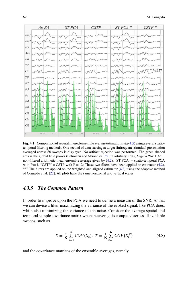
Fig. 4.1 Comparison of several filtered ensemble average estimations via (4.5) using several spatiotemporal filtering methods. One second of data starting at target (infrequent stimulus) presentation
averaged across 80 sweeps is displayed. No artifact rejection was performed. The green shaded
area is the global field power (Lehmann and Skrandies [52] in arbitrary units, Legend “Ar. EA”
non-filtered arithmetic mean ensemble average given by (4.2). “ST PCA” spatio-temporal PCA
with P 4. “CSTP” CSTP with P 12; These two filters have been applied to estimator (4.2).
“*” The filters are applied on the weighted and aligned estimator (4.3) using the adaptive method
of Congedo et al. [22]. All plots have the same horizontal and vertical scales
4.3.5 The Common Pattern
In order to improve upon the PCA we need to define a measure of the SNR, so that
we can devise a filter maximizing the variance of the evoked signal, like PCA does,
while also minimizing the variance of the noise. Consider the average spatial and
temporal sample covariance matrix when the average is computed across all available
sweeps, such as
S
1
K
K
k1
COV (X k ), T
1
K
K
k1
COV
X
T
k
(4.8)
and the covariance matrices of the ensemble averages, namely,
M. Congedo
Fig. 4.1 Comparison of several filtered ensemble average estimations via (4.5) using several spatiotemporal filtering methods. One second of data starting at target (infrequent stimulus) presentation
averaged across 80 sweeps is displayed. No artifact rejection was performed. The green shaded
area is the global field power (Lehmann and Skrandies [52] in arbitrary units, Legend “Ar. EA”
non-filtered arithmetic mean ensemble average given by (4.2). “ST PCA” spatio-temporal PCA
with P 4. “CSTP” CSTP with P 12; These two filters have been applied to estimator (4.2).
“*” The filters are applied on the weighted and aligned estimator (4.3) using the adaptive method
of Congedo et al. [22]. All plots have the same horizontal and vertical scales
4.3.5 The Common Pattern
In order to improve upon the PCA we need to define a measure of the SNR, so that
we can devise a filter maximizing the variance of the evoked signal, like PCA does,
while also minimizing the variance of the noise. Consider the average spatial and
temporal sample covariance matrix when the average is computed across all available
sweeps, such as
S
1
K
K
k1
COV (X k ), T
1
K
K
k1
COV
X
T
k
(4.8)
and the covariance matrices of the ensemble averages, namely,