

60
M. Congedo
⎧
⎪ ⎪ ⎨
⎪ ⎪ ⎩
¯
Y B
T ¯
X spatial
¯
Y ¯
X D temporal
¯
Y B
T ¯
X D spatio - temporal
.
(4.4)
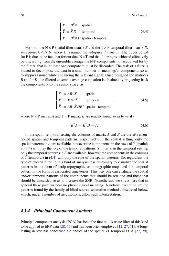
For both the N × P spatial filter matrix B and the T × P temporal filter matrix D,
we require 0 < P < N, where P is named the subspace dimension. The upper bound
for P is due to the fact that for our data N < T and that filtering is achieved effectively
by discarding from the ensemble average the N-P components not accounted for by
the filters, that is, at least one component must be discarded. The task of a filter is
indeed to decompose the data in a small number of meaningful components so as
to suppress noise while enhancing the relevant signal. Once designed the matrices
B and/or D, the filtered ensemble average estimation is obtained by projecting back
the components onto the sensor space, as
⎧
⎪ ⎪ ⎨
⎪ ⎪ ⎩
¯
X
AB
T ¯
X
spatial
¯
X
¯
X DE
T
temporal
¯
X
AB
T ¯
X DE
T spatio - temporal
,
(4.5)
where N × P matrix A and T × P matrix E are readily found so as to verify
B
T A E
T D I .
(4.6)
In the spatio-temporal setting the columns of matrix A and E are the aforementioned spatial and temporal patterns, respectively. In the spatial setting, only the
spatial patterns in A are available, however the components in the rows of ¯
Y (spatial)
in (4.4) will play the role of the temporal patterns. Similarly, in the temporal setting,
only the temporal patterns in E are available, however the components in the columns
of ¯
Y (temporal) in (4.4) will play the role of the spatial patterns. So, regardless the
type of chosen filter, in this kind of analysis it is customary to visualize the spatial
patterns in the form of scalp topographic or tomographic maps and the temporal
pattern in the form of associated time-series. This way one can evaluate the spatial
and/or temporal patterns of the components that should be retained and those that
should be discarded so as to increase the SNR. Nonetheless, we stress here that in
general these patterns bear no physiological meaning. A notable exception are the
patterns found by the family of blind source separation methods, discussed below,
which, under a number of assumptions, allow such interpretation.
4.3.4 Principal Component Analysis
Principal component analysis (PCA) has been the first multivariate filter of this kind
to be applied to ERP data [28, 45] and has been often employed [12, 27, 51]. A longlasting debate has concerned the choice of the spatial vs. temporal PCA [27, 79],
M. Congedo
⎧
⎪ ⎪ ⎨
⎪ ⎪ ⎩
¯
Y B
T ¯
X spatial
¯
Y ¯
X D temporal
¯
Y B
T ¯
X D spatio - temporal
.
(4.4)
For both the N × P spatial filter matrix B and the T × P temporal filter matrix D,
we require 0 < P < N, where P is named the subspace dimension. The upper bound
for P is due to the fact that for our data N < T and that filtering is achieved effectively
by discarding from the ensemble average the N-P components not accounted for by
the filters, that is, at least one component must be discarded. The task of a filter is
indeed to decompose the data in a small number of meaningful components so as
to suppress noise while enhancing the relevant signal. Once designed the matrices
B and/or D, the filtered ensemble average estimation is obtained by projecting back
the components onto the sensor space, as
⎧
⎪ ⎪ ⎨
⎪ ⎪ ⎩
¯
X
AB
T ¯
X
spatial
¯
X
¯
X DE
T
temporal
¯
X
AB
T ¯
X DE
T spatio - temporal
,
(4.5)
where N × P matrix A and T × P matrix E are readily found so as to verify
B
T A E
T D I .
(4.6)
In the spatio-temporal setting the columns of matrix A and E are the aforementioned spatial and temporal patterns, respectively. In the spatial setting, only the
spatial patterns in A are available, however the components in the rows of ¯
Y (spatial)
in (4.4) will play the role of the temporal patterns. Similarly, in the temporal setting,
only the temporal patterns in E are available, however the components in the columns
of ¯
Y (temporal) in (4.4) will play the role of the spatial patterns. So, regardless the
type of chosen filter, in this kind of analysis it is customary to visualize the spatial
patterns in the form of scalp topographic or tomographic maps and the temporal
pattern in the form of associated time-series. This way one can evaluate the spatial
and/or temporal patterns of the components that should be retained and those that
should be discarded so as to increase the SNR. Nonetheless, we stress here that in
general these patterns bear no physiological meaning. A notable exception are the
patterns found by the family of blind source separation methods, discussed below,
which, under a number of assumptions, allow such interpretation.
4.3.4 Principal Component Analysis
Principal component analysis (PCA) has been the first multivariate filter of this kind
to be applied to ERP data [28, 45] and has been often employed [12, 27, 51]. A longlasting debate has concerned the choice of the spatial vs. temporal PCA [27, 79],