

6 Methods for Functional Connectivity Analysis
131
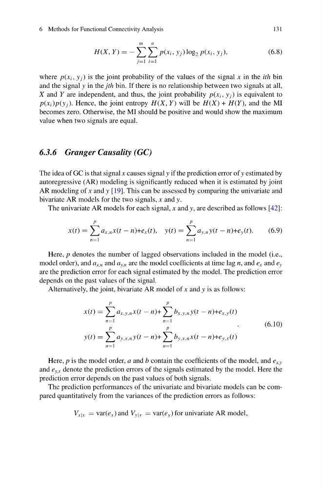
H (X, Y ) −
m
j1
n
i1
p(x i , y j ) log 2 p(x i , y j ),
(6.8)
where p(x i , y j ) is the joint probability of the values of the signal x in the ith bin
and the signal y in the jth bin. If there is no relationship between two signals at all,
X and Y are independent, and thus, the joint probability p(x i , y j ) is equivalent to
p(x i ) p(y j ). Hence, the joint entropy H (X, Y ) will be H (X ) + H (Y ), and the MI
becomes zero. Otherwise, the MI should be positive and would show the maximum
value when two signals are equal.
6.3.6 Granger Causality (GC)
The idea of GC is that signal x causes signal y if the prediction error of y estimated by
autoregressive (AR) modeling is significantly reduced when it is estimated by joint
AR modeling of x and y [19]. This can be assessed by comparing the univariate and
bivariate AR models for the two signals, x and y.
The univariate AR models for each signal, x and y, are described as follows [42]:
x(t)
p
n1
a x,n x(t − n)+e x (t), y(t)
p
n1
a y,n y(t − n)+e y (t).
(6.9)
Here, p denotes the number of lagged observations included in the model (i.e.,
model order), and a x,n and a y,n are the model coefficients at time lag n, and e x and e y
are the prediction error for each signal estimated by the model. The prediction error
depends on the past values of the signal.
Alternatively, the joint, bivariate AR model of x and y is as follows:
x(t)
p
n1
a x,y,n x(t − n)+
p
n1
b x,y,n y(t − n)+e x,y (t)
y(t)
p
n1
a y,x,n y(t − n)+
p
n1
b y,x,n x(t − n)+e y,x (t)
.
(6.10)
Here, p is the model order, a and b contain the coefficients of the model, and e x,y
and e y,x denote the prediction errors of the signals estimated by the model. Here the
prediction error depends on the past values of both signals.
The prediction performances of the univariate and bivariate models can be compared quantitatively from the variances of the prediction errors as follows:
V x|x var(e x ) and V y|y var(e y ) for univariate AR model,
131
H (X, Y ) −
m
j1
n
i1
p(x i , y j ) log 2 p(x i , y j ),
(6.8)
where p(x i , y j ) is the joint probability of the values of the signal x in the ith bin
and the signal y in the jth bin. If there is no relationship between two signals at all,
X and Y are independent, and thus, the joint probability p(x i , y j ) is equivalent to
p(x i ) p(y j ). Hence, the joint entropy H (X, Y ) will be H (X ) + H (Y ), and the MI
becomes zero. Otherwise, the MI should be positive and would show the maximum
value when two signals are equal.
6.3.6 Granger Causality (GC)
The idea of GC is that signal x causes signal y if the prediction error of y estimated by
autoregressive (AR) modeling is significantly reduced when it is estimated by joint
AR modeling of x and y [19]. This can be assessed by comparing the univariate and
bivariate AR models for the two signals, x and y.
The univariate AR models for each signal, x and y, are described as follows [42]:
x(t)
p
n1
a x,n x(t − n)+e x (t), y(t)
p
n1
a y,n y(t − n)+e y (t).
(6.9)
Here, p denotes the number of lagged observations included in the model (i.e.,
model order), and a x,n and a y,n are the model coefficients at time lag n, and e x and e y
are the prediction error for each signal estimated by the model. The prediction error
depends on the past values of the signal.
Alternatively, the joint, bivariate AR model of x and y is as follows:
x(t)
p
n1
a x,y,n x(t − n)+
p
n1
b x,y,n y(t − n)+e x,y (t)
y(t)
p
n1
a y,x,n y(t − n)+
p
n1
b y,x,n x(t − n)+e y,x (t)
.
(6.10)
Here, p is the model order, a and b contain the coefficients of the model, and e x,y
and e y,x denote the prediction errors of the signals estimated by the model. Here the
prediction error depends on the past values of both signals.
The prediction performances of the univariate and bivariate models can be compared quantitatively from the variances of the prediction errors as follows:
V x|x var(e x ) and V y|y var(e y ) for univariate AR model,