

112
Y. Zhang
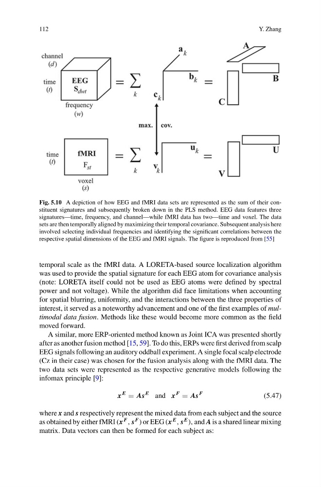
Fig. 5.10 A depiction of how EEG and fMRI data sets are represented as the sum of their constituent signatures and subsequently broken down in the PLS method. EEG data features three
signatures—time, frequency, and channel—while fMRI data has two—time and voxel. The data
sets are then temporally aligned by maximizing their temporal covariance. Subsequent analysis here
involved selecting individual frequencies and identifying the significant correlations between the
respective spatial dimensions of the EEG and fMRI signals. The figure is reproduced from [55]
temporal scale as the fMRI data. A LORETA-based source localization algorithm
was used to provide the spatial signature for each EEG atom for covariance analysis
(note: LORETA itself could not be used as EEG atoms were defined by spectral
power and not voltage). While the algorithm did face limitations when accounting
for spatial blurring, uniformity, and the interactions between the three properties of
interest, it served as a noteworthy advancement and one of the first examples of multimodal data fusion. Methods like these would become more common as the field
moved forward.
A similar, more ERP-oriented method known as Joint ICA was presented shortly
after as another fusion method [15, 59]. To do this, ERPs were first derived from scalp
EEG signals following an auditory oddball experiment. A single focal scalp electrode
(Cz in their case) was chosen for the fusion analysis along with the fMRI data. The
two data sets were represented as the respective generative models following the
infomax principle [9]:
x
E
As
E and x
F
As
F
(5.47)
where x and s respectively represent the mixed data from each subject and the source
as obtained by either fMRI (x
F
, s
F ) or EEG (x
E
, s
E ), and A is a shared linear mixing
matrix. Data vectors can then be formed for each subject as:
Y. Zhang
Fig. 5.10 A depiction of how EEG and fMRI data sets are represented as the sum of their constituent signatures and subsequently broken down in the PLS method. EEG data features three
signatures—time, frequency, and channel—while fMRI data has two—time and voxel. The data
sets are then temporally aligned by maximizing their temporal covariance. Subsequent analysis here
involved selecting individual frequencies and identifying the significant correlations between the
respective spatial dimensions of the EEG and fMRI signals. The figure is reproduced from [55]
temporal scale as the fMRI data. A LORETA-based source localization algorithm
was used to provide the spatial signature for each EEG atom for covariance analysis
(note: LORETA itself could not be used as EEG atoms were defined by spectral
power and not voltage). While the algorithm did face limitations when accounting
for spatial blurring, uniformity, and the interactions between the three properties of
interest, it served as a noteworthy advancement and one of the first examples of multimodal data fusion. Methods like these would become more common as the field
moved forward.
A similar, more ERP-oriented method known as Joint ICA was presented shortly
after as another fusion method [15, 59]. To do this, ERPs were first derived from scalp
EEG signals following an auditory oddball experiment. A single focal scalp electrode
(Cz in their case) was chosen for the fusion analysis along with the fMRI data. The
two data sets were represented as the respective generative models following the
infomax principle [9]:
x
E
As
E and x
F
As
F
(5.47)
where x and s respectively represent the mixed data from each subject and the source
as obtained by either fMRI (x
F
, s
F ) or EEG (x
E
, s
E ), and A is a shared linear mixing
matrix. Data vectors can then be formed for each subject as: