

5 EEG Source Imaging and Multimodal Neuroimaging
93
before the iterative process. With each iterative step requiring multiple calculations
of the forward solution using the test dipole(s), the least-squares method has a high
computational demand that is greatly increased when attempting to model multiple dipoles. To assuage this, several search methods have been commonly implemented—including the gradient, Nelder-Meade downhill search, multi-start simplex,
genetic algorithms [78]. Furthermore, the least-squares method faces two significant
drawbacks: (i) the solution with the minimum least-squares error is not necessarily
closest to the true underlying sources and (ii) The true number of active dipoles is
unknown and likely too large to be represented by a single “equivalent dipole”.
5.2.1.2 Beamforming Approaches
Another class of the parametric inverse solution is the beamforming methods. Unlike
the least-squares method, beamforming approaches do not search for equivalent
dipole(s) that fully explain the measured potentials. Instead, the contribution of a
single dipole source to the detected field is estimated, meaning that the number of
dipoles does not have to be assumed a priori. The beamformer acts as a spatial filter
that monitors the activity originating from one dipole source of interest and filters
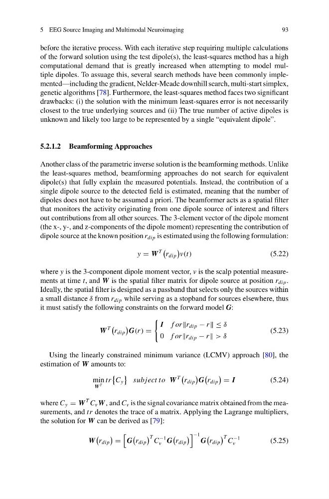
out contributions from all other sources. The 3-element vector of the dipole moment
(the x-, y-, and z-components of the dipole moment) representing the contribution of
dipole source at the known position r di p is estimated using the following formulation:
y W
T
r di p
v(t)
(5.22)
where y is the 3-component dipole moment vector, v is the scalp potential measurements at time t, and W is the spatial filter matrix for dipole source at position r di p .
Ideally, the spatial filter is designed as a passband that selects only the sources within
a small distance δ from r di p while serving as a stopband for sources elsewhere, thus
it must satisfy the following constraints on the forward model G:
W
T
r di p
G(r )
I f orr di p − r ≤ δ
0 f orr di p − r > δ
(5.23)
Using the linearly constrained minimum variance (LCMV) approach [80], the
estimation of W amounts to:
min
W
T
tr
C y
subject to W
T
r di p
G
r di p
I
(5.24)
where C y W
T C v W , and C v is the signal covariance matrix obtained from the measurements, and tr denotes the trace of a matrix. Applying the Lagrange multipliers,
the solution for W can be derived as [79]:
W
r di p
G
r di p
T C
−1
v G
r di p
−1
G
r di p
T C
−1
v
(5.25)
93
before the iterative process. With each iterative step requiring multiple calculations
of the forward solution using the test dipole(s), the least-squares method has a high
computational demand that is greatly increased when attempting to model multiple dipoles. To assuage this, several search methods have been commonly implemented—including the gradient, Nelder-Meade downhill search, multi-start simplex,
genetic algorithms [78]. Furthermore, the least-squares method faces two significant
drawbacks: (i) the solution with the minimum least-squares error is not necessarily
closest to the true underlying sources and (ii) The true number of active dipoles is
unknown and likely too large to be represented by a single “equivalent dipole”.
5.2.1.2 Beamforming Approaches
Another class of the parametric inverse solution is the beamforming methods. Unlike
the least-squares method, beamforming approaches do not search for equivalent
dipole(s) that fully explain the measured potentials. Instead, the contribution of a
single dipole source to the detected field is estimated, meaning that the number of
dipoles does not have to be assumed a priori. The beamformer acts as a spatial filter
that monitors the activity originating from one dipole source of interest and filters
out contributions from all other sources. The 3-element vector of the dipole moment
(the x-, y-, and z-components of the dipole moment) representing the contribution of
dipole source at the known position r di p is estimated using the following formulation:
y W
T
r di p
v(t)
(5.22)
where y is the 3-component dipole moment vector, v is the scalp potential measurements at time t, and W is the spatial filter matrix for dipole source at position r di p .
Ideally, the spatial filter is designed as a passband that selects only the sources within
a small distance δ from r di p while serving as a stopband for sources elsewhere, thus
it must satisfy the following constraints on the forward model G:
W
T
r di p
G(r )
I f orr di p − r ≤ δ
0 f orr di p − r > δ
(5.23)
Using the linearly constrained minimum variance (LCMV) approach [80], the
estimation of W amounts to:
min
W
T
tr
C y
subject to W
T
r di p
G
r di p
I
(5.24)
where C y W
T C v W , and C v is the signal covariance matrix obtained from the measurements, and tr denotes the trace of a matrix. Applying the Lagrange multipliers,
the solution for W can be derived as [79]:
W
r di p
G
r di p
T C
−1
v G
r di p
−1
G
r di p
T C
−1
v
(5.25)