

92
Y. Zhang
the estimated J. As such, the EEG inverse problem amounts to the calculation of
matrix M that would result in a satisfactory value for ˆ
J and the best fit with the
observed scalp potentials. The EEG inverse problem is an ill-posed problem due to
the non-uniqueness of its solution (the number of unknown sources is much larger
than the number of scalp measurements; P N ). To this end, there exists a number
of mathematical optimization schemes that provide solutions to the inverse problem
depending on the different configurations of the forward model. Specifically, different
assumptions can be made regarding the properties of the source space, such as the
number and/or the spatial distribution of the source current dipoles, and whether
the positions, magnitudes, and orientations of potential dipoles are fixed or varied.
Given the different forward model configurations, there are two main approaches to
the EEG inverse problem: parametric and non-parametric optimization methods.
5.2.1 Parametric Optimization Methods
In the family of parametric optimization methods, the source space usually comprises a single dipole or a few dipoles with unknown position(s), magnitude(s), and
orientation(s). These configurations are also known as equivalent current dipole
(ECD) models, wherein the solutions are obtained by searching for the “equivalent
dipole(s)” that best explain the observed scalp potentials. We present in the following
sections several popular representative methods for the EEG inverse problem of the
ECD model.
5.2.1.1 The Least-Squares Method
In a source model involving a single dipole, the solution can be obtained using the
non-linear least-squares method. This method solves for a single dipole with an
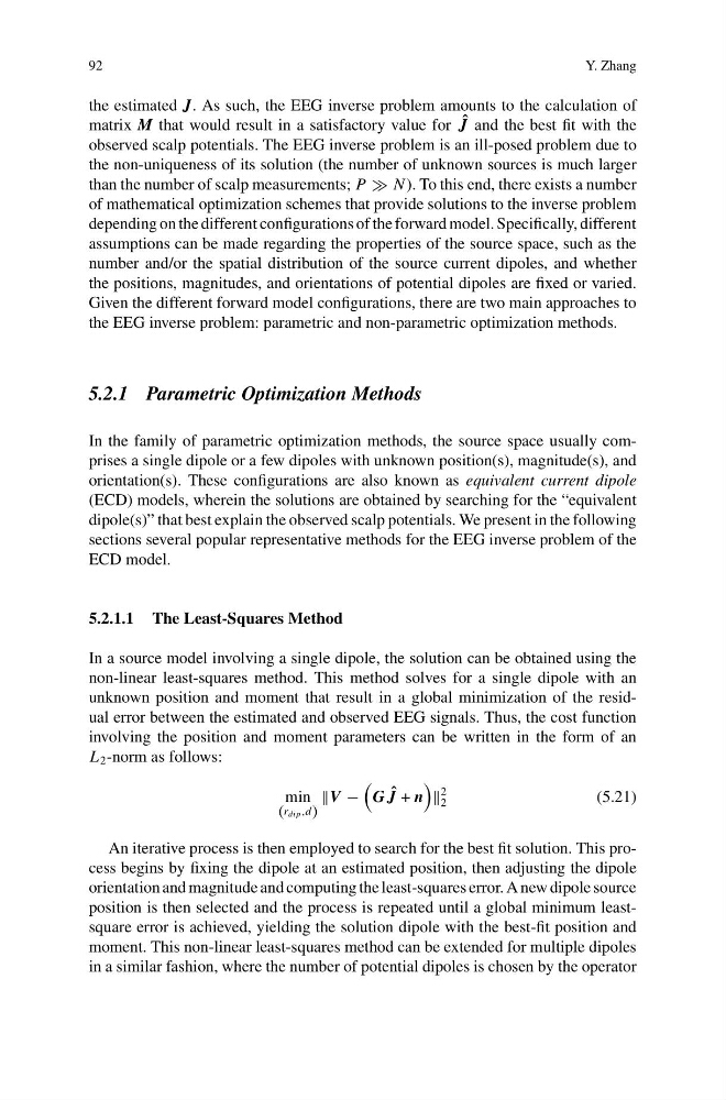
unknown position and moment that result in a global minimization of the residual error between the estimated and observed EEG signals. Thus, the cost function
involving the position and moment parameters can be written in the form of an
L 2 -norm as follows:
min
(rdip,d)
V −
G ˆ
J + n
2
2
(5.21)
An iterative process is then employed to search for the best fit solution. This process begins by fixing the dipole at an estimated position, then adjusting the dipole
orientation and magnitude and computing the least-squares error. A new dipole source
position is then selected and the process is repeated until a global minimum leastsquare error is achieved, yielding the solution dipole with the best-fit position and
moment. This non-linear least-squares method can be extended for multiple dipoles
in a similar fashion, where the number of potential dipoles is chosen by the operator
Y. Zhang
the estimated J. As such, the EEG inverse problem amounts to the calculation of
matrix M that would result in a satisfactory value for ˆ
J and the best fit with the
observed scalp potentials. The EEG inverse problem is an ill-posed problem due to
the non-uniqueness of its solution (the number of unknown sources is much larger
than the number of scalp measurements; P N ). To this end, there exists a number
of mathematical optimization schemes that provide solutions to the inverse problem
depending on the different configurations of the forward model. Specifically, different
assumptions can be made regarding the properties of the source space, such as the
number and/or the spatial distribution of the source current dipoles, and whether
the positions, magnitudes, and orientations of potential dipoles are fixed or varied.
Given the different forward model configurations, there are two main approaches to
the EEG inverse problem: parametric and non-parametric optimization methods.
5.2.1 Parametric Optimization Methods
In the family of parametric optimization methods, the source space usually comprises a single dipole or a few dipoles with unknown position(s), magnitude(s), and
orientation(s). These configurations are also known as equivalent current dipole
(ECD) models, wherein the solutions are obtained by searching for the “equivalent
dipole(s)” that best explain the observed scalp potentials. We present in the following
sections several popular representative methods for the EEG inverse problem of the
ECD model.
5.2.1.1 The Least-Squares Method
In a source model involving a single dipole, the solution can be obtained using the
non-linear least-squares method. This method solves for a single dipole with an
unknown position and moment that result in a global minimization of the residual error between the estimated and observed EEG signals. Thus, the cost function
involving the position and moment parameters can be written in the form of an
L 2 -norm as follows:
min
(rdip,d)
V −
G ˆ
J + n
2
2
(5.21)
An iterative process is then employed to search for the best fit solution. This process begins by fixing the dipole at an estimated position, then adjusting the dipole
orientation and magnitude and computing the least-squares error. A new dipole source
position is then selected and the process is repeated until a global minimum leastsquare error is achieved, yielding the solution dipole with the best-fit position and
moment. This non-linear least-squares method can be extended for multiple dipoles
in a similar fashion, where the number of potential dipoles is chosen by the operator