

determining tree form. A reduced form of the taper equation applied by Schneider
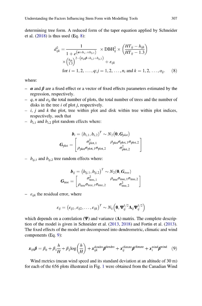
et al. (2018) is thus used (Eq. 8):
d
2
ijk ¼
1
1 þ e
αþb i, 1 þb ij, 1
ð
Þ
 DBH
2
ij Â
HT ij À h ijk
HT ij À 1:3
Â
h ijk
1:3
2À x ijk βþb i, 2 þb ij, 2
ð
Þ þ ε ijk
for i ¼ 1, 2, . . . , q; j ¼ 1, 2, . . . , n i and k ¼ 1, 2, . . . , o ij : ð8Þ
where:
– α and β are a fixed effect or a vector of fixed effects parameters estimated by the
regression, respectively.
– q, n and o ij the total number of plots, the total number of trees and the number of
disks in the tree i of plot j, respectively.
– i, j and k the plot, tree within plot and disk within tree within plot indices,
respectively, such that
– b i,1 and b i,2 plot random effects where:
b i ¼ b i, 1 ; b i, 2
ð
Þ
T $ N 2 0; G plot
À
Á
G plot ¼
σ
2
plot, 1
ρ plot σ plot, 1 σ plot, 2
ρ plot σ plot, 1 σ plot, 2
σ
2
plot, 2
"
#
– b ij,1 and b ij,2 tree random effects where:
b ij ¼ b ij, 1 ; b ij, 2
À
Á T $ N 2 0; G tree
ð
Þ
G tree ¼
σ
2
tree, 1
ρ tree σ tree, 1 σ tree, 2
ρ tree σ tree, 1 σ tree, 2
σ
2
tree, 2
!
– ε ijk the residual error, where
ε ij ¼ ε ij1 ; ε ij2 ; . . . ; ε ijk
À
Á T $ N k 0; Ψ
1=2
ij Λ ij Ψ
1=2
ij
which depends on a correlation (Ψ) and variance (Λ) matrix. The complete description of the model is given in Schneider et al. (2013, 2018) and Fortin et al. (2013).
The fixed effects of the model are decomposed into dendrometric, climatic and wind
components (Eq. 9):
x ijk β ¼ β 0 þ β 1
h
H
þ β 2 log
h
H
þ x
dendro
ijk
β
dendro
þ x
climate
ij
β
climate
þ x
wind
i
β
wind
ð9Þ
Wind metrics (mean wind speed and its standard deviation at an altitude of 30 m)
for each of the 656 plots illustrated in Fig. 1 were obtained from the Canadian Wind
Understanding the Factors Influencing Stem Form with Modelling Tools
307
et al. (2018) is thus used (Eq. 8):
d
2
ijk ¼
1
1 þ e
αþb i, 1 þb ij, 1
ð
Þ
 DBH
2
ij Â
HT ij À h ijk
HT ij À 1:3
Â
h ijk
1:3
2À x ijk βþb i, 2 þb ij, 2
ð
Þ þ ε ijk
for i ¼ 1, 2, . . . , q; j ¼ 1, 2, . . . , n i and k ¼ 1, 2, . . . , o ij : ð8Þ
where:
– α and β are a fixed effect or a vector of fixed effects parameters estimated by the
regression, respectively.
– q, n and o ij the total number of plots, the total number of trees and the number of
disks in the tree i of plot j, respectively.
– i, j and k the plot, tree within plot and disk within tree within plot indices,
respectively, such that
– b i,1 and b i,2 plot random effects where:
b i ¼ b i, 1 ; b i, 2
ð
Þ
T $ N 2 0; G plot
À
Á
G plot ¼
σ
2
plot, 1
ρ plot σ plot, 1 σ plot, 2
ρ plot σ plot, 1 σ plot, 2
σ
2
plot, 2
"
#
– b ij,1 and b ij,2 tree random effects where:
b ij ¼ b ij, 1 ; b ij, 2
À
Á T $ N 2 0; G tree
ð
Þ
G tree ¼
σ
2
tree, 1
ρ tree σ tree, 1 σ tree, 2
ρ tree σ tree, 1 σ tree, 2
σ
2
tree, 2
!
– ε ijk the residual error, where
ε ij ¼ ε ij1 ; ε ij2 ; . . . ; ε ijk
À
Á T $ N k 0; Ψ
1=2
ij Λ ij Ψ
1=2
ij
which depends on a correlation (Ψ) and variance (Λ) matrix. The complete description of the model is given in Schneider et al. (2013, 2018) and Fortin et al. (2013).
The fixed effects of the model are decomposed into dendrometric, climatic and wind
components (Eq. 9):
x ijk β ¼ β 0 þ β 1
h
H
þ β 2 log
h
H
þ x
dendro
ijk
β
dendro
þ x
climate
ij
β
climate
þ x
wind
i
β
wind
ð9Þ
Wind metrics (mean wind speed and its standard deviation at an altitude of 30 m)
for each of the 656 plots illustrated in Fig. 1 were obtained from the Canadian Wind
Understanding the Factors Influencing Stem Form with Modelling Tools
307