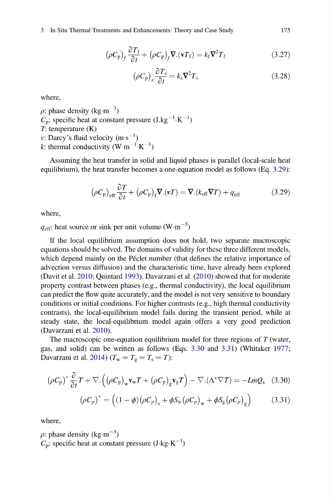
ρC p
À
Á
f
∂T f
∂t
þ ρC p
À
Á
f
—: vT f
ð Þ ¼ k f —
2 T f
ð3:27Þ
ρC p
À
Á
s
∂T s
∂t
¼ k s —
2 T s
ð3:28Þ
where,
ρ: phase density (kgÁm
À3 )
C p : specific heat at constant pressure (J.kg
À1
ÁK
À1 )
T: temperature (K)
v: Darcy’s fluid velocity (m∙s
À1 )
k: thermal conductivity (WÁm
À1
ÁK
À1 )
Assuming the heat transfer in solid and liquid phases is parallel (local-scale heat
equilibrium), the heat transfer becomes a one-equation model as follows (Eq. 3.29):
ρC p
À
Á
eff
∂T
∂t
þ ρC p
À
Á
f
—: vT
ð Þ ¼ —: k eff —T
ð
Þþq eff
ð3:29Þ
where,
q eff : heat source or sink per unit volume (WÁm
À3 )
If the local equilibrium assumption does not hold, two separate macroscopic
equations should be solved. The domains of validity for these three different models,
which depend mainly on the Péclet number (that defines the relative importance of
advection versus diffusion) and the characteristic time, have already been explored
(Davit et al. 2010; Quintard 1993). Davarzani et al. (2010) showed that for moderate
property contrast between phases (e.g., thermal conductivity), the local equilibrium
can predict the flow quite accurately, and the model is not very sensitive to boundary
conditions or initial conditions. For higher contrasts (e.g., high thermal conductivity
contrasts), the local-equilibrium model fails during the transient period, while at
steady state, the local-equilibrium model again offers a very good prediction
(Davarzani et al. 2010).
The macroscopic one-equation equilibrium model for three regions of T (water,
gas, and solid) can be written as follows (Eqs. 3.30 and 3.31) (Whitaker 1977;
Davarzani et al. 2014) (T w ¼ T g ¼ T s ¼ T ):
ρC p
À
Á Ã ∂
∂t
T þ ∇: ρC p
À
Á
w
v w T þ ρC p
À
Á
g
v g T
À ∇: Λ
Ã
∇T
ð
Þ¼ÀL _
mQ s ð3:30Þ
ρC p
À
Á Ã ¼ 1 À ϕ
ð
Þ ρC p
À
Á
s
þ ϕS w ρC p
À
Á
w
þ ϕS g ρC p
À
Á
g
ð3:31Þ
where,
ρ: phase density (kgÁm
À3 )
C p : specific heat at constant pressure (JÁkgÁK
À1 )
3 In Situ Thermal Treatments and Enhancements: Theory and Case Study
175