

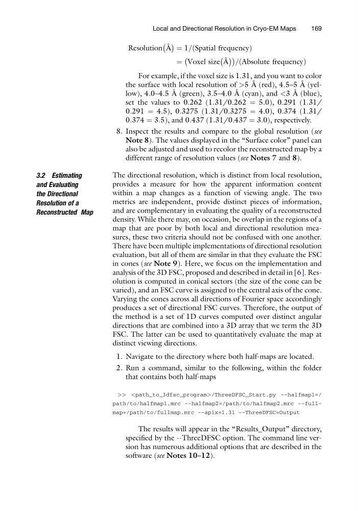
Resolution Å
À Á ¼ 1= Spatial frequency
ð
Þ
¼ Voxel size Å
À Á
À
Á = Absolute frequency
ð
Þ
For example, if the voxel size is 1.31, and you want to color
the surface with local resolution of >5 Å (red), 4.5–5 Å (yellow), 4.0–4.5 Å (green), 3.5–4.0 Å (cyan), and <3 Å (blue),
set the values to 0.262 (1.31/0.262 ¼ 5.0), 0.291 (1.31/
0.291 ¼ 4.5), 0.3275 (1.31/0.3275 ¼ 4.0), 0.374 (1.31/
0.374 ¼ 3.5), and 0.437 (1.31/0.437 ¼ 3.0), respectively.
8. Inspect the results and compare to the global resolution (see
Note 8). The values displayed in the “Surface color” panel can
also be adjusted and used to recolor the reconstructed map by a
different range of resolution values (see Notes 7 and 8).
3.2 Estimating
and Evaluating
the Directional
Resolution of a
Reconstructed Map
The directional resolution, which is distinct from local resolution,
provides a measure for how the apparent information content
within a map changes as a function of viewing angle. The two
metrics are independent, provide distinct pieces of information,
and are complementary in evaluating the quality of a reconstructed
density. While there may, on occasion, be overlap in the regions of a
map that are poor by both local and directional resolution measures, these two criteria should not be confused with one another.
There have been multiple implementations of directional resolution
evaluation, but all of them are similar in that they evaluate the FSC
in cones (see Note 9). Here, we focus on the implementation and
analysis of the 3D FSC, proposed and described in detail in [6]. Resolution is computed in conical sectors (the size of the cone can be
varied), and an FSC curve is assigned to the central axis of the cone.
Varying the cones across all directions of Fourier space accordingly
produces a set of directional FSC curves. Therefore, the output of
the method is a set of 1D curves computed over distinct angular
directions that are combined into a 3D array that we term the 3D
FSC. The latter can be used to quantitatively evaluate the map at
distinct viewing directions.
1. Navigate to the directory where both half-maps are located.
2. Run a command, similar to the following, within the folder
that contains both half-maps
>>/ThreeDFSC_Start.py --halfmap1=/
path/to/halfmap1.mrc --halfmap2=/path/to/halfmap2.mrc --fullmap=/path/to/fullmap.mrc --apix=1.31 --ThreeDFSC=Output
The results will appear in the “Results_Output” directory,
specified by the --ThreeDFSC option. The command line version has numerous additional options that are described in the
software (see Notes 10–12).
Local and Directional Resolution in Cryo-EM Maps
169
À Á ¼ 1= Spatial frequency
ð
Þ
¼ Voxel size Å
À Á
À
Á = Absolute frequency
ð
Þ
For example, if the voxel size is 1.31, and you want to color
the surface with local resolution of >5 Å (red), 4.5–5 Å (yellow), 4.0–4.5 Å (green), 3.5–4.0 Å (cyan), and <3 Å (blue),
set the values to 0.262 (1.31/0.262 ¼ 5.0), 0.291 (1.31/
0.291 ¼ 4.5), 0.3275 (1.31/0.3275 ¼ 4.0), 0.374 (1.31/
0.374 ¼ 3.5), and 0.437 (1.31/0.437 ¼ 3.0), respectively.
8. Inspect the results and compare to the global resolution (see
Note 8). The values displayed in the “Surface color” panel can
also be adjusted and used to recolor the reconstructed map by a
different range of resolution values (see Notes 7 and 8).
3.2 Estimating
and Evaluating
the Directional
Resolution of a
Reconstructed Map
The directional resolution, which is distinct from local resolution,
provides a measure for how the apparent information content
within a map changes as a function of viewing angle. The two
metrics are independent, provide distinct pieces of information,
and are complementary in evaluating the quality of a reconstructed
density. While there may, on occasion, be overlap in the regions of a
map that are poor by both local and directional resolution measures, these two criteria should not be confused with one another.
There have been multiple implementations of directional resolution
evaluation, but all of them are similar in that they evaluate the FSC
in cones (see Note 9). Here, we focus on the implementation and
analysis of the 3D FSC, proposed and described in detail in [6]. Resolution is computed in conical sectors (the size of the cone can be
varied), and an FSC curve is assigned to the central axis of the cone.
Varying the cones across all directions of Fourier space accordingly
produces a set of directional FSC curves. Therefore, the output of
the method is a set of 1D curves computed over distinct angular
directions that are combined into a 3D array that we term the 3D
FSC. The latter can be used to quantitatively evaluate the map at
distinct viewing directions.
1. Navigate to the directory where both half-maps are located.
2. Run a command, similar to the following, within the folder
that contains both half-maps
>>
path/to/halfmap1.mrc --halfmap2=/path/to/halfmap2.mrc --fullmap=/path/to/fullmap.mrc --apix=1.31 --ThreeDFSC=Output
The results will appear in the “Results_Output” directory,
specified by the --ThreeDFSC option. The command line version has numerous additional options that are described in the
software (see Notes 10–12).
Local and Directional Resolution in Cryo-EM Maps
169