

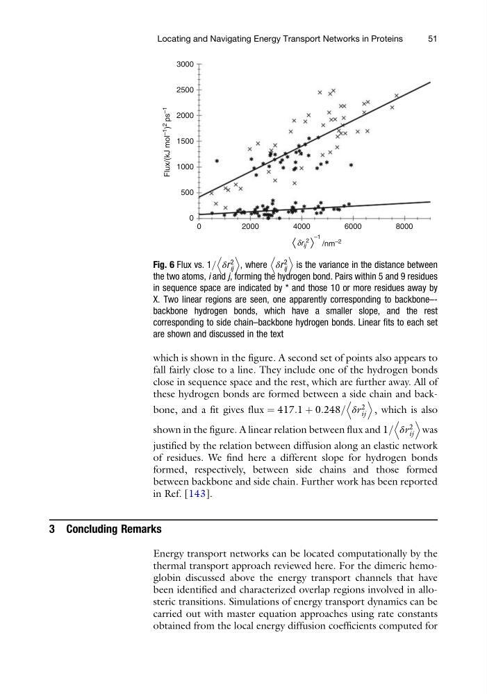
which is shown in the figure. A second set of points also appears to
fall fairly close to a line. They include one of the hydrogen bonds
close in sequence space and the rest, which are further away. All of
these hydrogen bonds are formed between a side chain and backbone, and a fit gives flux ¼ 417:1 þ 0:248= δr
2
ij
D
E
, which is also
shown in the figure. A linear relation between flux and 1= δr
2
ij
D
E
was
justified by the relation between diffusion along an elastic network
of residues. We find here a different slope for hydrogen bonds
formed, respectively, between side chains and those formed
between backbone and side chain. Further work has been reported
in Ref. [143].
3 Concluding Remarks
Energy transport networks can be located computationally by the
thermal transport approach reviewed here. For the dimeric hemoglobin discussed above the energy transport channels that have
been identified and characterized overlap regions involved in allosteric transitions. Simulations of energy transport dynamics can be
carried out with master equation approaches using rate constants
obtained from the local energy diffusion coefficients computed for
0
2000
Flux/(kJ mol
–1
)
2
ps
–1
4000
/nm
–2
–1
〈dr ij
2
6000
8000
0
500
1000
1500
2000
2500
3000
〉
Fig. 6 Flux vs. 1= δr
2
ij
D E
, where δr
2
ij
D E
is the variance in the distance between
the two atoms, i and j, forming the hydrogen bond. Pairs within 5 and 9 residues
in sequence space are indicated by * and those 10 or more residues away by
X. Two linear regions are seen, one apparently corresponding to backbone–backbone hydrogen bonds, which have a smaller slope, and the rest
corresponding to side chain–backbone hydrogen bonds. Linear fits to each set
are shown and discussed in the text
Locating and Navigating Energy Transport Networks in Proteins
51
fall fairly close to a line. They include one of the hydrogen bonds
close in sequence space and the rest, which are further away. All of
these hydrogen bonds are formed between a side chain and backbone, and a fit gives flux ¼ 417:1 þ 0:248= δr
2
ij
D
E
, which is also
shown in the figure. A linear relation between flux and 1= δr
2
ij
D
E
was
justified by the relation between diffusion along an elastic network
of residues. We find here a different slope for hydrogen bonds
formed, respectively, between side chains and those formed
between backbone and side chain. Further work has been reported
in Ref. [143].
3 Concluding Remarks
Energy transport networks can be located computationally by the
thermal transport approach reviewed here. For the dimeric hemoglobin discussed above the energy transport channels that have
been identified and characterized overlap regions involved in allosteric transitions. Simulations of energy transport dynamics can be
carried out with master equation approaches using rate constants
obtained from the local energy diffusion coefficients computed for
0
2000
Flux/(kJ mol
–1
)
2
ps
–1
4000
/nm
–2
–1
〈dr ij
2
6000
8000
0
500
1000
1500
2000
2500
3000
〉
Fig. 6 Flux vs. 1= δr
2
ij
D E
, where δr
2
ij
D E
is the variance in the distance between
the two atoms, i and j, forming the hydrogen bond. Pairs within 5 and 9 residues
in sequence space are indicated by * and those 10 or more residues away by
X. Two linear regions are seen, one apparently corresponding to backbone–backbone hydrogen bonds, which have a smaller slope, and the rest
corresponding to side chain–backbone hydrogen bonds. Linear fits to each set
are shown and discussed in the text
Locating and Navigating Energy Transport Networks in Proteins
51