

296
References
Ackleson SG, Klemas V (1987) Remote sensing of submerged aquatic vegetation in lower
Chesapeake Bay: a comparison of Landsat MSS to TM imagery. Remote Sens Environ 22:235–
248. https://doi.org/10.1016/0034-4257(87)90060-5
Albright TP, Moorhouse TG, Mcnabb TJ (2004) The rise and fall of water hyacinth in Lake Victoria
and the Kagera river basin. J Aquat Plant Manage 42:73–84
Ali I, Cawkwell F, Dwyer E et al (2016) Satellite remote sensing of grasslands: from observation
to management. J Plant Ecol 9:649–671. https://doi.org/10.1093/jpe/rtw005
Allen JM, Bradley BA (2016) Out of the weeds? Reduced plant invasion risk with climate
change in the continental United States. Biol Conserv 203:306–312. https://doi.org/10.1016/j.
biocon.2016.09.015
Alonzo M, Bookhagen B, Roberts DA (2014) Urban tree species mapping using hyperspectral and
lidar data fusion. Remote Sens Environ 148:70–83. https://doi.org/10.1016/j.rse.2014.03.018
Amaral CH, Roberts DA, Almeida TIR, Souza Filho CR (2015) Mapping invasive species and
spectral mixture relationships with neotropical woody formations in southeastern Brazil.
ISPRS J Photogramm Remote Sens 108:80–93. https://doi.org/10.1016/j.isprsjprs.2015.06.009
Anderson JM (1991) The effects of climate change on decomposition processes in grassland and
coniferous forests. Ecol Appl 1:326–347. https://doi.org/10.2307/1941761
Anderson GL, Hanson JD, Haas RH (1993) Evaluating landsat thematic mapper derived vegetation indices for estimating above-ground biomass on semiarid rangelands. Remote Sens
Environ 45:165–175. https://doi.org/10.1016/0034-4257(93)90040-5
Anderson DM, Glibert PM, Burkholder JM (2002) Harmful algal blooms and eutrophication: nutrient sources, composition, and consequences. Estuaries 25:704–726. https://doi.org/10.1007/
bf02804901
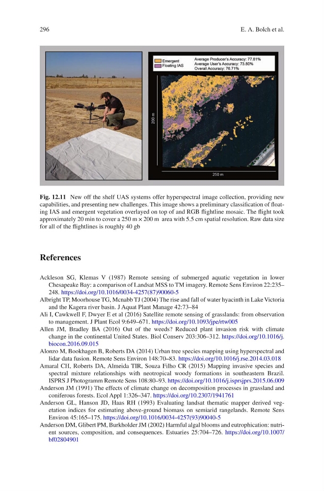
Fig. 12.11 New off the shelf UAS systems offer hyperspectral image collection, providing new
capabilities, and presenting new challenges. This image shows a preliminary classification of floating IAS and emergent vegetation overlayed on top of and RGB flightline mosaic. The flight took
approximately 20 min to cover a 250 m × 200 m area with 5.5 cm spatial resolution. Raw data size
for all of the flightlines is roughly 40 gb
E. A. Bolch et al.
References
Ackleson SG, Klemas V (1987) Remote sensing of submerged aquatic vegetation in lower
Chesapeake Bay: a comparison of Landsat MSS to TM imagery. Remote Sens Environ 22:235–
248. https://doi.org/10.1016/0034-4257(87)90060-5
Albright TP, Moorhouse TG, Mcnabb TJ (2004) The rise and fall of water hyacinth in Lake Victoria
and the Kagera river basin. J Aquat Plant Manage 42:73–84
Ali I, Cawkwell F, Dwyer E et al (2016) Satellite remote sensing of grasslands: from observation
to management. J Plant Ecol 9:649–671. https://doi.org/10.1093/jpe/rtw005
Allen JM, Bradley BA (2016) Out of the weeds? Reduced plant invasion risk with climate
change in the continental United States. Biol Conserv 203:306–312. https://doi.org/10.1016/j.
biocon.2016.09.015
Alonzo M, Bookhagen B, Roberts DA (2014) Urban tree species mapping using hyperspectral and
lidar data fusion. Remote Sens Environ 148:70–83. https://doi.org/10.1016/j.rse.2014.03.018
Amaral CH, Roberts DA, Almeida TIR, Souza Filho CR (2015) Mapping invasive species and
spectral mixture relationships with neotropical woody formations in southeastern Brazil.
ISPRS J Photogramm Remote Sens 108:80–93. https://doi.org/10.1016/j.isprsjprs.2015.06.009
Anderson JM (1991) The effects of climate change on decomposition processes in grassland and
coniferous forests. Ecol Appl 1:326–347. https://doi.org/10.2307/1941761
Anderson GL, Hanson JD, Haas RH (1993) Evaluating landsat thematic mapper derived vegetation indices for estimating above-ground biomass on semiarid rangelands. Remote Sens
Environ 45:165–175. https://doi.org/10.1016/0034-4257(93)90040-5
Anderson DM, Glibert PM, Burkholder JM (2002) Harmful algal blooms and eutrophication: nutrient sources, composition, and consequences. Estuaries 25:704–726. https://doi.org/10.1007/
bf02804901
Fig. 12.11 New off the shelf UAS systems offer hyperspectral image collection, providing new
capabilities, and presenting new challenges. This image shows a preliminary classification of floating IAS and emergent vegetation overlayed on top of and RGB flightline mosaic. The flight took
approximately 20 min to cover a 250 m × 200 m area with 5.5 cm spatial resolution. Raw data size
for all of the flightlines is roughly 40 gb
E. A. Bolch et al.