

240
diversity was calculated as the aggregated effective species number of all plots
within a 50 km radius of the focal plot, including the focal plot. For each 50 km
radius centered on a focal plot, we computed the standard deviation of elevation
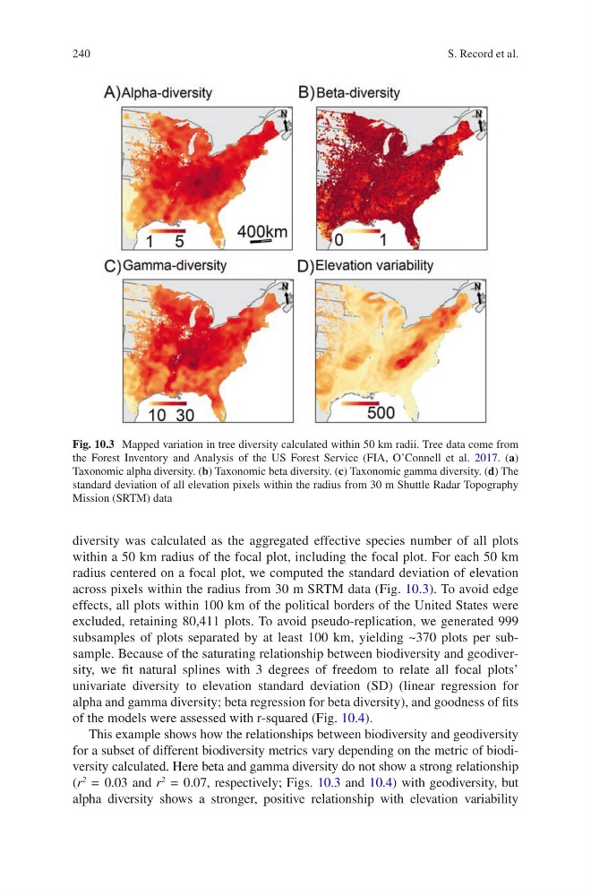
across pixels within the radius from 30 m SRTM data (Fig. 10.3). To avoid edge
effects, all plots within 100 km of the political borders of the United States were
excluded, retaining 80,411 plots. To avoid pseudo-replication, we generated 999
subsamples of plots separated by at least 100 km, yielding ~370 plots per subsample. Because of the saturating relationship between biodiversity and geodiversity, we fit natural splines with 3 degrees of freedom to relate all focal plots’
univariate diversity to elevation standard deviation (SD) (linear regression for
alpha and gamma diversity; beta regression for beta diversity), and goodness of fits
of the models were assessed with r-squared (Fig. 10.4).
This example shows how the relationships between biodiversity and geodiversity
for a subset of different biodiversity metrics vary depending on the metric of biodiversity calculated. Here beta and gamma diversity do not show a strong relationship
(r
2
= 0.03 and r
2
= 0.07, respectively; Figs. 10.3 and 10.4) with geodiversity, but
alpha diversity shows a stronger, positive relationship with elevation variability
Fig. 10.3 Mapped variation in tree diversity calculated within 50 km radii. Tree data come from
the Forest Inventory and Analysis of the US Forest Service (FIA, O’Connell et al. 2017. (a)
Taxonomic alpha diversity. (b) Taxonomic beta diversity. (c) Taxonomic gamma diversity. (d) The
standard deviation of all elevation pixels within the radius from 30 m Shuttle Radar Topography
Mission (SRTM) data
S. Record et al.
diversity was calculated as the aggregated effective species number of all plots
within a 50 km radius of the focal plot, including the focal plot. For each 50 km
radius centered on a focal plot, we computed the standard deviation of elevation
across pixels within the radius from 30 m SRTM data (Fig. 10.3). To avoid edge
effects, all plots within 100 km of the political borders of the United States were
excluded, retaining 80,411 plots. To avoid pseudo-replication, we generated 999
subsamples of plots separated by at least 100 km, yielding ~370 plots per subsample. Because of the saturating relationship between biodiversity and geodiversity, we fit natural splines with 3 degrees of freedom to relate all focal plots’
univariate diversity to elevation standard deviation (SD) (linear regression for
alpha and gamma diversity; beta regression for beta diversity), and goodness of fits
of the models were assessed with r-squared (Fig. 10.4).
This example shows how the relationships between biodiversity and geodiversity
for a subset of different biodiversity metrics vary depending on the metric of biodiversity calculated. Here beta and gamma diversity do not show a strong relationship
(r
2
= 0.03 and r
2
= 0.07, respectively; Figs. 10.3 and 10.4) with geodiversity, but
alpha diversity shows a stronger, positive relationship with elevation variability
Fig. 10.3 Mapped variation in tree diversity calculated within 50 km radii. Tree data come from
the Forest Inventory and Analysis of the US Forest Service (FIA, O’Connell et al. 2017. (a)
Taxonomic alpha diversity. (b) Taxonomic beta diversity. (c) Taxonomic gamma diversity. (d) The
standard deviation of all elevation pixels within the radius from 30 m Shuttle Radar Topography
Mission (SRTM) data
S. Record et al.