

232
Ruggedness Index (TRI), in contrast, is the mean of the difference between the
central pixel and its surrounding pixels (Riley et al. 1999). Wood (1996) describes a
number of convexity and curvature metrics based on the first and second derivatives
of the quadratic surface described above. DEMs can also be classified into topographic features or landforms like peaks, ridges, channels, and pits, though these
definitions depend on specific threshold values that may either be prescribed by
software or defined by the user. Incident solar radiation can also be calculated for a
given day or aggregated for a year based on a given point’s elevation and latitude
and the elevations of surrounding pixels. Although this section mainly describes
DEM-derived morphometric landforms, it is also important to acknowledge that the
genesis of landforms interacts with the ecology of a system. For instance, two hills
with similar shapes may have very different associated vegetation if one is sandy
(e.g., a dune) and the other is made of tills (e.g., end moraine).
While SRTM-derived products are typically used to produce “best available”
topographic information, a challenge with SRTM is that the mission occurred
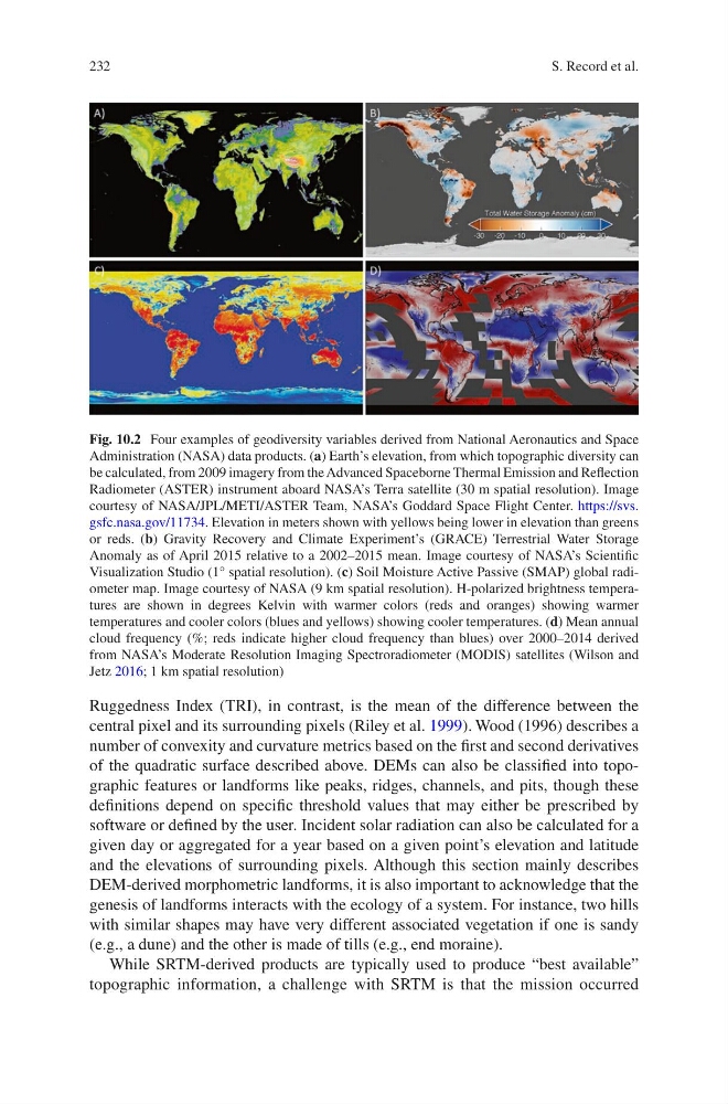
Fig. 10.2 Four examples of geodiversity variables derived from National Aeronautics and Space
Administration (NASA) data products. (a) Earth’s elevation, from which topographic diversity can
be calculated, from 2009 imagery from the Advanced Spaceborne Thermal Emission and Reflection
Radiometer (ASTER) instrument aboard NASA’s Terra satellite (30 m spatial resolution). Image
courtesy of NASA/JPL/METI/ASTER Team, NASA’s Goddard Space Flight Center. https://svs.
gsfc.nasa.gov/11734. Elevation in meters shown with yellows being lower in elevation than greens
or reds. (b) Gravity Recovery and Climate Experiment’s (GRACE) Terrestrial Water Storage
Anomaly as of April 2015 relative to a 2002–2015 mean. Image courtesy of NASA’s Scientific
Visualization Studio (1° spatial resolution). (c) Soil Moisture Active Passive (SMAP) global radiometer map. Image courtesy of NASA (9 km spatial resolution). H-polarized brightness temperatures are shown in degrees Kelvin with warmer colors (reds and oranges) showing warmer
temperatures and cooler colors (blues and yellows) showing cooler temperatures. (d) Mean annual
cloud frequency (%; reds indicate higher cloud frequency than blues) over 2000–2014 derived
from NASA’s Moderate Resolution Imaging Spectroradiometer (MODIS) satellites (Wilson and
Jetz 2016; 1 km spatial resolution)
S. Record et al.
Ruggedness Index (TRI), in contrast, is the mean of the difference between the
central pixel and its surrounding pixels (Riley et al. 1999). Wood (1996) describes a
number of convexity and curvature metrics based on the first and second derivatives
of the quadratic surface described above. DEMs can also be classified into topographic features or landforms like peaks, ridges, channels, and pits, though these
definitions depend on specific threshold values that may either be prescribed by
software or defined by the user. Incident solar radiation can also be calculated for a
given day or aggregated for a year based on a given point’s elevation and latitude
and the elevations of surrounding pixels. Although this section mainly describes
DEM-derived morphometric landforms, it is also important to acknowledge that the
genesis of landforms interacts with the ecology of a system. For instance, two hills
with similar shapes may have very different associated vegetation if one is sandy
(e.g., a dune) and the other is made of tills (e.g., end moraine).
While SRTM-derived products are typically used to produce “best available”
topographic information, a challenge with SRTM is that the mission occurred
Fig. 10.2 Four examples of geodiversity variables derived from National Aeronautics and Space
Administration (NASA) data products. (a) Earth’s elevation, from which topographic diversity can
be calculated, from 2009 imagery from the Advanced Spaceborne Thermal Emission and Reflection
Radiometer (ASTER) instrument aboard NASA’s Terra satellite (30 m spatial resolution). Image
courtesy of NASA/JPL/METI/ASTER Team, NASA’s Goddard Space Flight Center. https://svs.
gsfc.nasa.gov/11734. Elevation in meters shown with yellows being lower in elevation than greens
or reds. (b) Gravity Recovery and Climate Experiment’s (GRACE) Terrestrial Water Storage
Anomaly as of April 2015 relative to a 2002–2015 mean. Image courtesy of NASA’s Scientific
Visualization Studio (1° spatial resolution). (c) Soil Moisture Active Passive (SMAP) global radiometer map. Image courtesy of NASA (9 km spatial resolution). H-polarized brightness temperatures are shown in degrees Kelvin with warmer colors (reds and oranges) showing warmer
temperatures and cooler colors (blues and yellows) showing cooler temperatures. (d) Mean annual
cloud frequency (%; reds indicate higher cloud frequency than blues) over 2000–2014 derived
from NASA’s Moderate Resolution Imaging Spectroradiometer (MODIS) satellites (Wilson and
Jetz 2016; 1 km spatial resolution)
S. Record et al.