

210
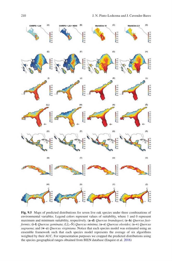
Fig. 9.5 Maps of predicted distributions for seven live oak species under three combinations of
environmental variables. Legend colors represent values of suitability, where 1 and 0 represent
maximum and minimum suitability, respectively. (a–d) Quercus brandegeei; (e–h) Quercus fusiformis; (i–l) Quercus geminata; (LL–Ñ) Quercus minima; (o–r) Quercus oleoides; (s–v) Quercus
sagraena; and (w–z) Quercus virginiana. Notice that each species model was estimated using an
ensemble framework such that each species model represents the average of six algorithms
weighted by their AUC. For representation purposes we cropped the predicted distributions using
the species geographical ranges obtained from BIEN database (Enquist et al. 2016)
J. N. Pinto-Ledezma and J. Cavender-Bares
Fig. 9.5 Maps of predicted distributions for seven live oak species under three combinations of
environmental variables. Legend colors represent values of suitability, where 1 and 0 represent
maximum and minimum suitability, respectively. (a–d) Quercus brandegeei; (e–h) Quercus fusiformis; (i–l) Quercus geminata; (LL–Ñ) Quercus minima; (o–r) Quercus oleoides; (s–v) Quercus
sagraena; and (w–z) Quercus virginiana. Notice that each species model was estimated using an
ensemble framework such that each species model represents the average of six algorithms
weighted by their AUC. For representation purposes we cropped the predicted distributions using
the species geographical ranges obtained from BIEN database (Enquist et al. 2016)
J. N. Pinto-Ledezma and J. Cavender-Bares