

Raw FLIM data are analyzed by obtaining excited-state
lifetime values first on a pixel-by-pixel basis, then of a region
of interest, and calculations are made using SPCImage analysis
software.
7. The distribution of lifetime values within the region of interest
is generated and displayed as a curve. Only chi-squared (χ
2 )
values between 0.9 and 1.3 are considered a good fit of the data
points. For a pure sample such as the test solutions and donor
FPs (mTurq2 or YFP), it is best to fit the data to a singleexponential decay. The median, minimum, and maximum
values of the lifetime values from the curve are taken to generate the range of lifetimes per sample. At least three areas of a
sample dish and at least three independent biological samples
per protein–protein combination are analyzed and the average
of the ranges is taken. The percentage efficiency of energy
transfer (E) from one protein to the other may be determined
using Eqs. (1) and (2):
E% ¼ 1 À
τ DA
τ D
 100
ð5Þ
where τ D and τ DA are the measured excited-state lifetime of the
donor and acceptor, respectively.
3.9 Typical Results
Typical multichannel FLIM results of multiple protein interactions
are shown in Fig. 4 and changes in lifetime values are given in
Table 6.
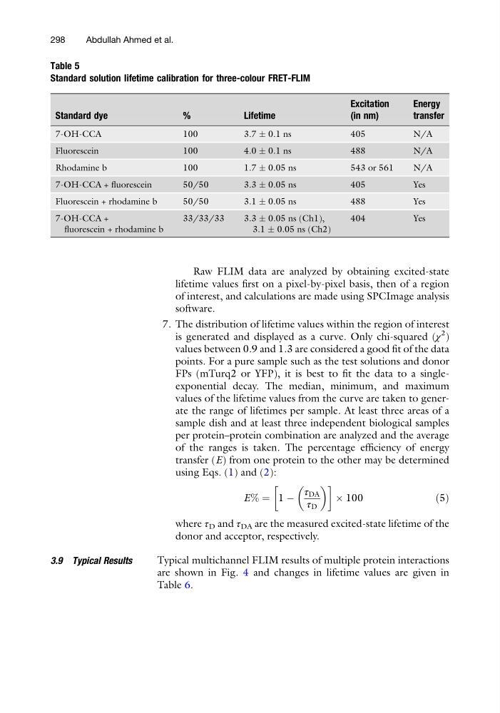
Table 5
Standard solution lifetime calibration for three-colour FRET-FLIM
Standard dye
%
Lifetime
Excitation
(in nm)
Energy
transfer
7-OH-CCA
100
3.7 Æ 0.1 ns
405
N/A
Fluorescein
100
4.0 Æ 0.1 ns
488
N/A
Rhodamine b
100
1.7 Æ 0.05 ns
543 or 561
N/A
7-OH-CCA + fluorescein
50/50
3.3 Æ 0.05 ns
405
Yes
Fluorescein + rhodamine b
50/50
3.1 Æ 0.05 ns
488
Yes
7-OH-CCA +
fluorescein + rhodamine b
33/33/33
3.3 Æ 0.05 ns (Ch1),
3.1 Æ 0.05 ns (Ch2)
404
Yes
298
Abdullah Ahmed et al.
lifetime values first on a pixel-by-pixel basis, then of a region
of interest, and calculations are made using SPCImage analysis
software.
7. The distribution of lifetime values within the region of interest
is generated and displayed as a curve. Only chi-squared (χ
2 )
values between 0.9 and 1.3 are considered a good fit of the data
points. For a pure sample such as the test solutions and donor
FPs (mTurq2 or YFP), it is best to fit the data to a singleexponential decay. The median, minimum, and maximum
values of the lifetime values from the curve are taken to generate the range of lifetimes per sample. At least three areas of a
sample dish and at least three independent biological samples
per protein–protein combination are analyzed and the average
of the ranges is taken. The percentage efficiency of energy
transfer (E) from one protein to the other may be determined
using Eqs. (1) and (2):
E% ¼ 1 À
τ DA
τ D
 100
ð5Þ
where τ D and τ DA are the measured excited-state lifetime of the
donor and acceptor, respectively.
3.9 Typical Results
Typical multichannel FLIM results of multiple protein interactions
are shown in Fig. 4 and changes in lifetime values are given in
Table 6.
Table 5
Standard solution lifetime calibration for three-colour FRET-FLIM
Standard dye
%
Lifetime
Excitation
(in nm)
Energy
transfer
7-OH-CCA
100
3.7 Æ 0.1 ns
405
N/A
Fluorescein
100
4.0 Æ 0.1 ns
488
N/A
Rhodamine b
100
1.7 Æ 0.05 ns
543 or 561
N/A
7-OH-CCA + fluorescein
50/50
3.3 Æ 0.05 ns
405
Yes
Fluorescein + rhodamine b
50/50
3.1 Æ 0.05 ns
488
Yes
7-OH-CCA +
fluorescein + rhodamine b
33/33/33
3.3 Æ 0.05 ns (Ch1),
3.1 Æ 0.05 ns (Ch2)
404
Yes
298
Abdullah Ahmed et al.