

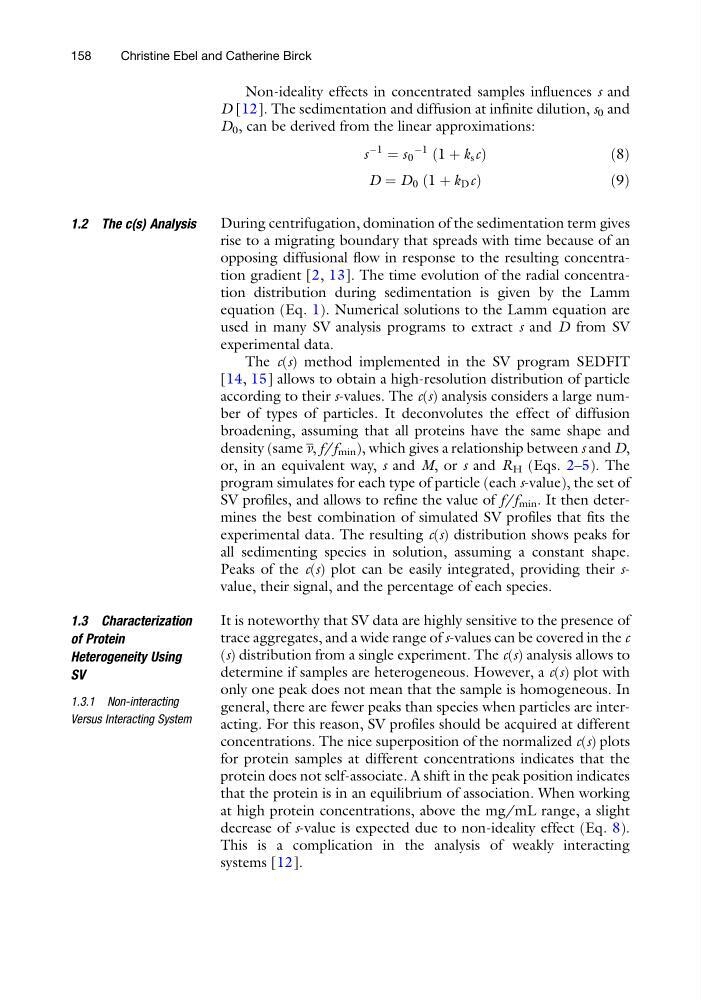
Non-ideality effects in concentrated samples influences s and
D [12]. The sedimentation and diffusion at infinite dilution, s 0 and
D 0 , can be derived from the linear approximations:
s
À1
¼ s 0
À1 1 þ k s c
ð
Þ
ð8Þ
D ¼ D 0 1 þ k D c
ð
Þ
ð 9Þ
1.2 The c(s) Analysis
During centrifugation, domination of the sedimentation term gives
rise to a migrating boundary that spreads with time because of an
opposing diffusional flow in response to the resulting concentration gradient [2, 13]. The time evolution of the radial concentration distribution during sedimentation is given by the Lamm
equation (Eq. 1). Numerical solutions to the Lamm equation are
used in many SV analysis programs to extract s and D from SV
experimental data.
The c(s) method implemented in the SV program SEDFIT
[14, 15] allows to obtain a high-resolution distribution of particle
according to their s-values. The c(s) analysis considers a large number of types of particles. It deconvolutes the effect of diffusion
broadening, assuming that all proteins have the same shape and
density (same v, f/f min ), which gives a relationship between s and D,
or, in an equivalent way, s and M, or s and R H (Eqs. 2–5). The
program simulates for each type of particle (each s-value), the set of
SV profiles, and allows to refine the value of f/f min . It then determines the best combination of simulated SV profiles that fits the
experimental data. The resulting c(s) distribution shows peaks for
all sedimenting species in solution, assuming a constant shape.
Peaks of the c(s) plot can be easily integrated, providing their svalue, their signal, and the percentage of each species.
1.3 Characterization
of Protein
Heterogeneity Using
SV
1.3.1 Non-interacting
Versus Interacting System
It is noteworthy that SV data are highly sensitive to the presence of
trace aggregates, and a wide range of s-values can be covered in the c
(s) distribution from a single experiment. The c(s) analysis allows to
determine if samples are heterogeneous. However, a c(s) plot with
only one peak does not mean that the sample is homogeneous. In
general, there are fewer peaks than species when particles are interacting. For this reason, SV profiles should be acquired at different
concentrations. The nice superposition of the normalized c(s) plots
for protein samples at different concentrations indicates that the
protein does not self-associate. A shift in the peak position indicates
that the protein is in an equilibrium of association. When working
at high protein concentrations, above the mg/mL range, a slight
decrease of s-value is expected due to non-ideality effect (Eq. 8).
This is a complication in the analysis of weakly interacting
systems [12].
158
Christine Ebel and Catherine Birck
D [12]. The sedimentation and diffusion at infinite dilution, s 0 and
D 0 , can be derived from the linear approximations:
s
À1
¼ s 0
À1 1 þ k s c
ð
Þ
ð8Þ
D ¼ D 0 1 þ k D c
ð
Þ
ð 9Þ
1.2 The c(s) Analysis
During centrifugation, domination of the sedimentation term gives
rise to a migrating boundary that spreads with time because of an
opposing diffusional flow in response to the resulting concentration gradient [2, 13]. The time evolution of the radial concentration distribution during sedimentation is given by the Lamm
equation (Eq. 1). Numerical solutions to the Lamm equation are
used in many SV analysis programs to extract s and D from SV
experimental data.
The c(s) method implemented in the SV program SEDFIT
[14, 15] allows to obtain a high-resolution distribution of particle
according to their s-values. The c(s) analysis considers a large number of types of particles. It deconvolutes the effect of diffusion
broadening, assuming that all proteins have the same shape and
density (same v, f/f min ), which gives a relationship between s and D,
or, in an equivalent way, s and M, or s and R H (Eqs. 2–5). The
program simulates for each type of particle (each s-value), the set of
SV profiles, and allows to refine the value of f/f min . It then determines the best combination of simulated SV profiles that fits the
experimental data. The resulting c(s) distribution shows peaks for
all sedimenting species in solution, assuming a constant shape.
Peaks of the c(s) plot can be easily integrated, providing their svalue, their signal, and the percentage of each species.
1.3 Characterization
of Protein
Heterogeneity Using
SV
1.3.1 Non-interacting
Versus Interacting System
It is noteworthy that SV data are highly sensitive to the presence of
trace aggregates, and a wide range of s-values can be covered in the c
(s) distribution from a single experiment. The c(s) analysis allows to
determine if samples are heterogeneous. However, a c(s) plot with
only one peak does not mean that the sample is homogeneous. In
general, there are fewer peaks than species when particles are interacting. For this reason, SV profiles should be acquired at different
concentrations. The nice superposition of the normalized c(s) plots
for protein samples at different concentrations indicates that the
protein does not self-associate. A shift in the peak position indicates
that the protein is in an equilibrium of association. When working
at high protein concentrations, above the mg/mL range, a slight
decrease of s-value is expected due to non-ideality effect (Eq. 8).
This is a complication in the analysis of weakly interacting
systems [12].
158
Christine Ebel and Catherine Birck