

To cover all tilt angles (180° or p) with the given step size, the number of images
required is:
m ¼
p
Da
¼ p
D
d
Note that for a single tilt series, this equation only accounts for a limit on
resolution perpendicular to the tilt axis. It also assumes noise-free images in perfect
alignment. Noise and alignment errors will suppress the resolution. Targeting a
particular number of images for a tilt series is in practice more a function of the total
dose desired than the achievable resolution based on the Crowther criterion.
The most appropriate way of considering resolution in a full tomogram is to
assess the recovery of information from each image in the tilt series. Cardone et al.
[69] devised a method called noise-compensated leave-one-out (NLOO). The
method calculates for each micrograph the ratio between two Fourier ring correlations (FRCs): the first an FRC between the micrograph and a projection from the
full reconstruction with the micrograph left out, and the second an FRC between the
micrograph and a projection from the full reconstruction. This is however only
applicable to integrative methods (WBP and FSR), because the iterative methods
incorporate a similar comparison already in the reconstruction.
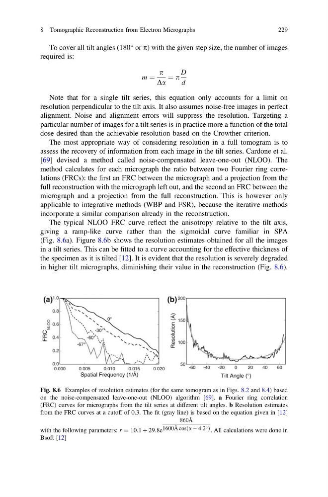
The typical NLOO FRC curve reflect the anisotropy relative to the tilt axis,
giving a ramp-like curve rather than the sigmoidal curve familiar in SPA
(Fig. 8.6a). Figure 8.6b shows the resolution estimates obtained for all the images
in a tilt series. This can be fitted to a curve accounting for the effective thickness of
the specimen as it is tilted [12]. It is evident that the resolution is severely degraded
in higher tilt micrographs, diminishing their value in the reconstruction (Fig. 8.6).
Fig. 8.6 Examples of resolution estimates (for the same tomogram as in Figs. 8.2 and 8.4) based
on the noise-compensated leave-one-out (NLOO) algorithm [69]. a Fourier ring correlation
(FRC) curves for micrographs from the tilt series at different tilt angles. b Resolution estimates
from the FRC curves at a cutoff of 0.3. The fit (gray line) is based on the equation given in [12]
with the following parameters: r ¼ 10:1 þ 29:8e
860 ˚
A
1600 ˚
A cosða À 4:2 Þ . All calculations were done in
Bsoft [12]
8 Tomographic Reconstruction from Electron Micrographs
229
required is:
m ¼
p
Da
¼ p
D
d
Note that for a single tilt series, this equation only accounts for a limit on
resolution perpendicular to the tilt axis. It also assumes noise-free images in perfect
alignment. Noise and alignment errors will suppress the resolution. Targeting a
particular number of images for a tilt series is in practice more a function of the total
dose desired than the achievable resolution based on the Crowther criterion.
The most appropriate way of considering resolution in a full tomogram is to
assess the recovery of information from each image in the tilt series. Cardone et al.
[69] devised a method called noise-compensated leave-one-out (NLOO). The
method calculates for each micrograph the ratio between two Fourier ring correlations (FRCs): the first an FRC between the micrograph and a projection from the
full reconstruction with the micrograph left out, and the second an FRC between the
micrograph and a projection from the full reconstruction. This is however only
applicable to integrative methods (WBP and FSR), because the iterative methods
incorporate a similar comparison already in the reconstruction.
The typical NLOO FRC curve reflect the anisotropy relative to the tilt axis,
giving a ramp-like curve rather than the sigmoidal curve familiar in SPA
(Fig. 8.6a). Figure 8.6b shows the resolution estimates obtained for all the images
in a tilt series. This can be fitted to a curve accounting for the effective thickness of
the specimen as it is tilted [12]. It is evident that the resolution is severely degraded
in higher tilt micrographs, diminishing their value in the reconstruction (Fig. 8.6).
Fig. 8.6 Examples of resolution estimates (for the same tomogram as in Figs. 8.2 and 8.4) based
on the noise-compensated leave-one-out (NLOO) algorithm [69]. a Fourier ring correlation
(FRC) curves for micrographs from the tilt series at different tilt angles. b Resolution estimates
from the FRC curves at a cutoff of 0.3. The fit (gray line) is based on the equation given in [12]
with the following parameters: r ¼ 10:1 þ 29:8e
860 ˚
A
1600 ˚
A cosða À 4:2 Þ . All calculations were done in
Bsoft [12]
8 Tomographic Reconstruction from Electron Micrographs
229