

angle. The complication is that the defocus contains both these real and frequency
space terms. Therefore, the convolution theorem cannot be used to simplify the
calculation of the power spectrum or correcting for the CTF.
8.5.2 Determining CTF Parameters
To determine the CTF parameters (defocus average, defocus deviation and astigmatism angle), a representative power spectrum must be calculated. This is commonly done by dividing the image into tiles and averaging the power spectra of the
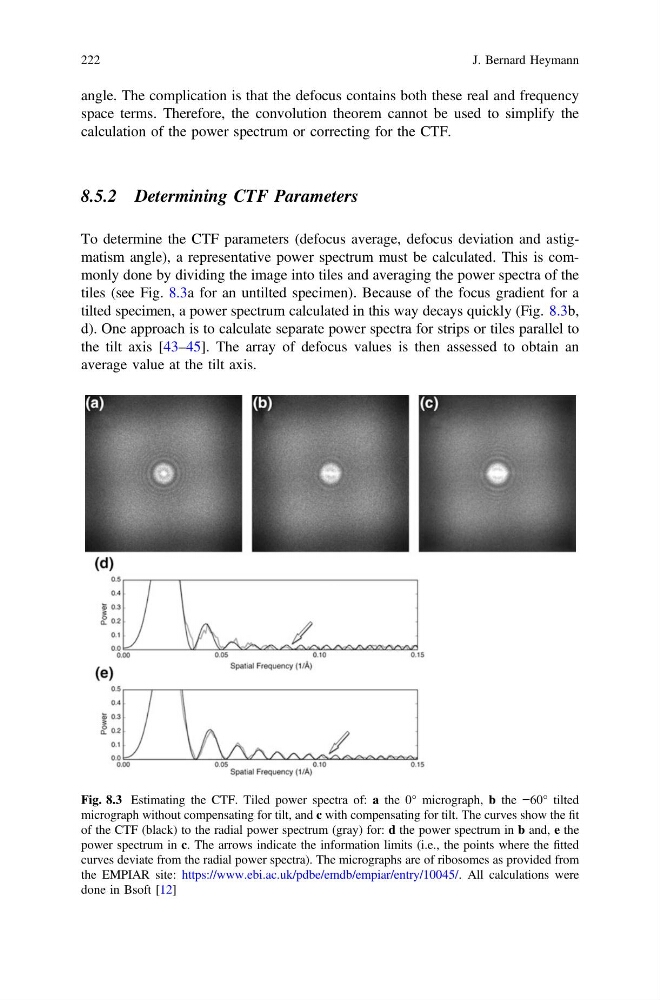
tiles (see Fig. 8.3a for an untilted specimen). Because of the focus gradient for a
tilted specimen, a power spectrum calculated in this way decays quickly (Fig. 8.3b,
d). One approach is to calculate separate power spectra for strips or tiles parallel to
the tilt axis [43–45]. The array of defocus values is then assessed to obtain an
average value at the tilt axis.
Fig. 8.3 Estimating the CTF. Tiled power spectra of: a the 0° micrograph, b the −60° tilted
micrograph without compensating for tilt, and c with compensating for tilt. The curves show the fit
of the CTF (black) to the radial power spectrum (gray) for: d the power spectrum in b and, e the
power spectrum in c. The arrows indicate the information limits (i.e., the points where the fitted
curves deviate from the radial power spectra). The micrographs are of ribosomes as provided from
the EMPIAR site: https://www.ebi.ac.uk/pdbe/emdb/empiar/entry/10045/. All calculations were
done in Bsoft [12]
222
J. Bernard Heymann
space terms. Therefore, the convolution theorem cannot be used to simplify the
calculation of the power spectrum or correcting for the CTF.
8.5.2 Determining CTF Parameters
To determine the CTF parameters (defocus average, defocus deviation and astigmatism angle), a representative power spectrum must be calculated. This is commonly done by dividing the image into tiles and averaging the power spectra of the
tiles (see Fig. 8.3a for an untilted specimen). Because of the focus gradient for a
tilted specimen, a power spectrum calculated in this way decays quickly (Fig. 8.3b,
d). One approach is to calculate separate power spectra for strips or tiles parallel to
the tilt axis [43–45]. The array of defocus values is then assessed to obtain an
average value at the tilt axis.
Fig. 8.3 Estimating the CTF. Tiled power spectra of: a the 0° micrograph, b the −60° tilted
micrograph without compensating for tilt, and c with compensating for tilt. The curves show the fit
of the CTF (black) to the radial power spectrum (gray) for: d the power spectrum in b and, e the
power spectrum in c. The arrows indicate the information limits (i.e., the points where the fitted
curves deviate from the radial power spectra). The micrographs are of ribosomes as provided from
the EMPIAR site: https://www.ebi.ac.uk/pdbe/emdb/empiar/entry/10045/. All calculations were
done in Bsoft [12]
222
J. Bernard Heymann