

pixel and the destination voxel. The source image can be padded in real space to
increase the sampling in frequency space, thus decreasing the distance between source
and destination grid points [12].
The natural interpolation in frequency space is of the Whittaker-Shannon type,
based on sinc functions [9, 13, 14]. Exact interpolation (such as Whittaker-Shannon)
implicitly assumes that the data is noise-less and that the continuous function can be
reconstructed exactly up to Nyquest frequency. However, with significant noise
present, the reconstruction with exact interpolation will emphasize the noise rather
than the embedded signal. The smoothing effect of approximate interpolation
methods such as nearest neighbor and bilinear interpolation has yielded acceptable
results in the presence of noise.
Gridded-based interpolation is an approximation aimed at changing the sampling
grid in frequency space. An intermediate sampling grid is often not rectangular,
constructed through variations of fast Fourier transformation (FFT) called unequally
spaced FFT (USFFT) [15] or non-uniform FFT (NUFFT) [16]. Several iterative
forms of interpolation have been developed to improve accuracy [16–18]. It is not
clear in practice that the slight increases in accuracy of gridded-based interpolation
[42] is worth the more complicated implementation.
8.3 Iterative Reconstruction
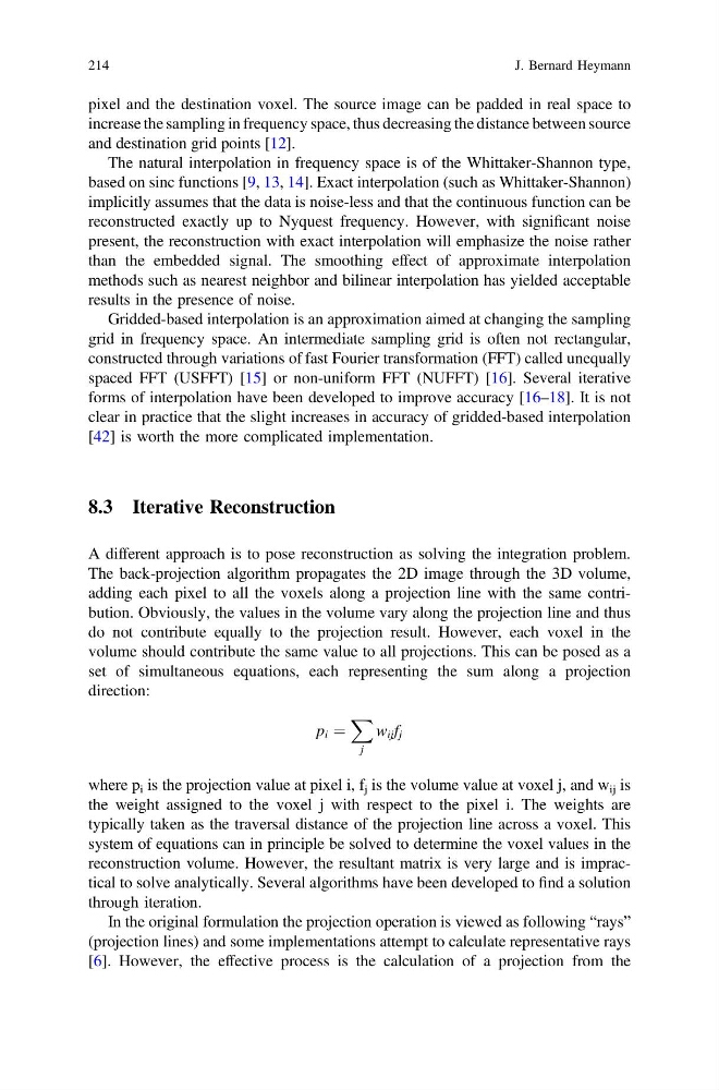
A different approach is to pose reconstruction as solving the integration problem.
The back-projection algorithm propagates the 2D image through the 3D volume,
adding each pixel to all the voxels along a projection line with the same contribution. Obviously, the values in the volume vary along the projection line and thus
do not contribute equally to the projection result. However, each voxel in the
volume should contribute the same value to all projections. This can be posed as a
set of simultaneous equations, each representing the sum along a projection
direction:
p i ¼
X
j
w ij f j
where p i is the projection value at pixel i, f j is the volume value at voxel j, and w ij is
the weight assigned to the voxel j with respect to the pixel i. The weights are
typically taken as the traversal distance of the projection line across a voxel. This
system of equations can in principle be solved to determine the voxel values in the
reconstruction volume. However, the resultant matrix is very large and is impractical to solve analytically. Several algorithms have been developed to find a solution
through iteration.
In the original formulation the projection operation is viewed as following “rays”
(projection lines) and some implementations attempt to calculate representative rays
[6]. However, the effective process is the calculation of a projection from the
214
J. Bernard Heymann
increase the sampling in frequency space, thus decreasing the distance between source
and destination grid points [12].
The natural interpolation in frequency space is of the Whittaker-Shannon type,
based on sinc functions [9, 13, 14]. Exact interpolation (such as Whittaker-Shannon)
implicitly assumes that the data is noise-less and that the continuous function can be
reconstructed exactly up to Nyquest frequency. However, with significant noise
present, the reconstruction with exact interpolation will emphasize the noise rather
than the embedded signal. The smoothing effect of approximate interpolation
methods such as nearest neighbor and bilinear interpolation has yielded acceptable
results in the presence of noise.
Gridded-based interpolation is an approximation aimed at changing the sampling
grid in frequency space. An intermediate sampling grid is often not rectangular,
constructed through variations of fast Fourier transformation (FFT) called unequally
spaced FFT (USFFT) [15] or non-uniform FFT (NUFFT) [16]. Several iterative
forms of interpolation have been developed to improve accuracy [16–18]. It is not
clear in practice that the slight increases in accuracy of gridded-based interpolation
[42] is worth the more complicated implementation.
8.3 Iterative Reconstruction
A different approach is to pose reconstruction as solving the integration problem.
The back-projection algorithm propagates the 2D image through the 3D volume,
adding each pixel to all the voxels along a projection line with the same contribution. Obviously, the values in the volume vary along the projection line and thus
do not contribute equally to the projection result. However, each voxel in the
volume should contribute the same value to all projections. This can be posed as a
set of simultaneous equations, each representing the sum along a projection
direction:
p i ¼
X
j
w ij f j
where p i is the projection value at pixel i, f j is the volume value at voxel j, and w ij is
the weight assigned to the voxel j with respect to the pixel i. The weights are
typically taken as the traversal distance of the projection line across a voxel. This
system of equations can in principle be solved to determine the voxel values in the
reconstruction volume. However, the resultant matrix is very large and is impractical to solve analytically. Several algorithms have been developed to find a solution
through iteration.
In the original formulation the projection operation is viewed as following “rays”
(projection lines) and some implementations attempt to calculate representative rays
[6]. However, the effective process is the calculation of a projection from the
214
J. Bernard Heymann