

account for the fact that the two images being compared are coming from the same
3D object and are related by a single tilt operation. However, let us give one step
back and introduce the correlation as a measure of similarity between two images.
Let us assume that we have two identical images whose relationship between
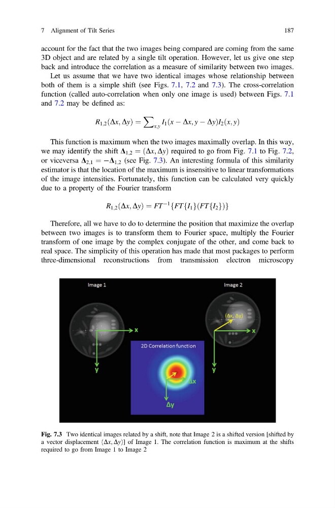
both of them is a simple shift (see Figs. 7.1, 7.2 and 7.3). The cross-correlation
function (called auto-correlation when only one image is used) between Figs. 7.1
and 7.2 may be defined as:
R 1;2 Dx; Dy
ð
Þ¼
X
x;y
I 1 x À Dx; y À Dy
ð
Þ I 2 x; y
ð Þ
This function is maximum when the two images maximally overlap. In this way,
we may identify the shift D 1;2 ¼ Dx; Dy
ð
Þrequired to go from Fig. 7.1 to Fig. 7.2,
or viceversa D 2;1 ¼ ÀD 1;2 (see Fig. 7.3). An interesting formula of this similarity
estimator is that the location of the maximum is insensitive to linear transformations
of the image intensities. Fortunately, this function can be calculated very quickly
due to a property of the Fourier transform
R 1;2 Dx; Dy
ð
Þ¼FT
À1
fFT I 1
f gðFT I 2
f gÞg
Therefore, all we have to do to determine the position that maximize the overlap
between two images is to transform them to Fourier space, multiply the Fourier
transform of one image by the complex conjugate of the other, and come back to
real space. The simplicity of this operation has made that most packages to perform
three-dimensional reconstructions from transmission electron microscopy
Fig. 7.3 Two identical images related by a shift, note that Image 2 is a shifted version [shifted by
a vector displacement Dx; Dy
ð
Þ ] of Image 1. The correlation function is maximum at the shifts
required to go from Image 1 to Image 2
7 Alignment of Tilt Series
187
3D object and are related by a single tilt operation. However, let us give one step
back and introduce the correlation as a measure of similarity between two images.
Let us assume that we have two identical images whose relationship between
both of them is a simple shift (see Figs. 7.1, 7.2 and 7.3). The cross-correlation
function (called auto-correlation when only one image is used) between Figs. 7.1
and 7.2 may be defined as:
R 1;2 Dx; Dy
ð
Þ¼
X
x;y
I 1 x À Dx; y À Dy
ð
Þ I 2 x; y
ð Þ
This function is maximum when the two images maximally overlap. In this way,
we may identify the shift D 1;2 ¼ Dx; Dy
ð
Þrequired to go from Fig. 7.1 to Fig. 7.2,
or viceversa D 2;1 ¼ ÀD 1;2 (see Fig. 7.3). An interesting formula of this similarity
estimator is that the location of the maximum is insensitive to linear transformations
of the image intensities. Fortunately, this function can be calculated very quickly
due to a property of the Fourier transform
R 1;2 Dx; Dy
ð
Þ¼FT
À1
fFT I 1
f gðFT I 2
f gÞg
Therefore, all we have to do to determine the position that maximize the overlap
between two images is to transform them to Fourier space, multiply the Fourier
transform of one image by the complex conjugate of the other, and come back to
real space. The simplicity of this operation has made that most packages to perform
three-dimensional reconstructions from transmission electron microscopy
Fig. 7.3 Two identical images related by a shift, note that Image 2 is a shifted version [shifted by
a vector displacement Dx; Dy
ð
Þ ] of Image 1. The correlation function is maximum at the shifts
required to go from Image 1 to Image 2
7 Alignment of Tilt Series
187