

54
P. Sjödin et al.
PC
% Variation explained
0
2
4
6
10
12
8
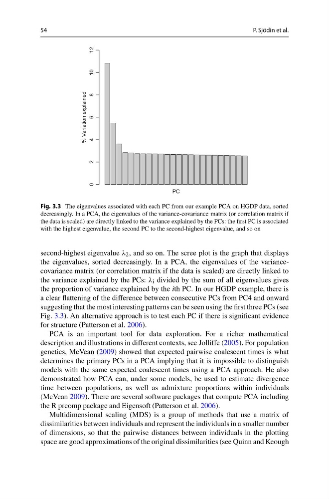
Fig. 3.3 The eigenvalues associated with each PC from our example PCA on HGDP data, sorted
decreasingly. In a PCA, the eigenvalues of the variance-covariance matrix (or correlation matrix if
the data is scaled) are directly linked to the variance explained by the PCs: the first PC is associated
with the highest eigenvalue, the second PC to the second-highest eigenvalue, and so on
second-highest eigenvalue λ 2 , and so on. The scree plot is the graph that displays
the eigenvalues, sorted decreasingly. In a PCA, the eigenvalues of the variancecovariance matrix (or correlation matrix if the data is scaled) are directly linked to
the variance explained by the PCs: λ i divided by the sum of all eigenvalues gives
the proportion of variance explained by the ith PC. In our HGDP example, there is
a clear flattening of the difference between consecutive PCs from PC4 and onward
suggesting that the most interesting patterns can be seen using the first three PCs (see
Fig. 3.3). An alternative approach is to test each PC if there is significant evidence
for structure (Patterson et al. 2006).
PCA is an important tool for data exploration. For a richer mathematical
description and illustrations in different contexts, see Jolliffe (2005). For population
genetics, McVean (2009) showed that expected pairwise coalescent times is what
determines the primary PCs in a PCA implying that it is impossible to distinguish
models with the same expected coalescent times using a PCA approach. He also
demonstrated how PCA can, under some models, be used to estimate divergence
time between populations, as well as admixture proportions within individuals
(McVean 2009). There are several software packages that compute PCA including
the R prcomp package and Eigensoft (Patterson et al. 2006).
Multidimensional scaling (MDS) is a group of methods that use a matrix of
dissimilarities between individuals and represent the individuals in a smaller number
of dimensions, so that the pairwise distances between individuals in the plotting
space are good approximations of the original dissimilarities (see Quinn and Keough
P. Sjödin et al.
PC
% Variation explained
0
2
4
6
10
12
8
Fig. 3.3 The eigenvalues associated with each PC from our example PCA on HGDP data, sorted
decreasingly. In a PCA, the eigenvalues of the variance-covariance matrix (or correlation matrix if
the data is scaled) are directly linked to the variance explained by the PCs: the first PC is associated
with the highest eigenvalue, the second PC to the second-highest eigenvalue, and so on
second-highest eigenvalue λ 2 , and so on. The scree plot is the graph that displays
the eigenvalues, sorted decreasingly. In a PCA, the eigenvalues of the variancecovariance matrix (or correlation matrix if the data is scaled) are directly linked to
the variance explained by the PCs: λ i divided by the sum of all eigenvalues gives
the proportion of variance explained by the ith PC. In our HGDP example, there is
a clear flattening of the difference between consecutive PCs from PC4 and onward
suggesting that the most interesting patterns can be seen using the first three PCs (see
Fig. 3.3). An alternative approach is to test each PC if there is significant evidence
for structure (Patterson et al. 2006).
PCA is an important tool for data exploration. For a richer mathematical
description and illustrations in different contexts, see Jolliffe (2005). For population
genetics, McVean (2009) showed that expected pairwise coalescent times is what
determines the primary PCs in a PCA implying that it is impossible to distinguish
models with the same expected coalescent times using a PCA approach. He also
demonstrated how PCA can, under some models, be used to estimate divergence
time between populations, as well as admixture proportions within individuals
(McVean 2009). There are several software packages that compute PCA including
the R prcomp package and Eigensoft (Patterson et al. 2006).
Multidimensional scaling (MDS) is a group of methods that use a matrix of
dissimilarities between individuals and represent the individuals in a smaller number
of dimensions, so that the pairwise distances between individuals in the plotting
space are good approximations of the original dissimilarities (see Quinn and Keough