

3 Analysis of Population Structure
53
−0.2
−0.1
0.0
0.1
0.2
−0.2
−0.1
0.0
0.1
0.2
0.3
PC1: 10.817 %
PC2: 5.484 %
San
French
Mozabite
Yoruba
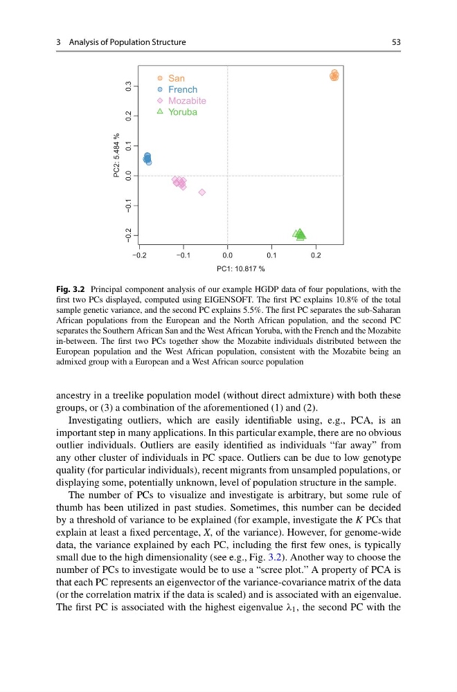
Fig. 3.2 Principal component analysis of our example HGDP data of four populations, with the
first two PCs displayed, computed using EIGENSOFT. The first PC explains 10.8% of the total
sample genetic variance, and the second PC explains 5.5%. The first PC separates the sub-Saharan
African populations from the European and the North African population, and the second PC
separates the Southern African San and the West African Yoruba, with the French and the Mozabite
in-between. The first two PCs together show the Mozabite individuals distributed between the
European population and the West African population, consistent with the Mozabite being an
admixed group with a European and a West African source population
ancestry in a treelike population model (without direct admixture) with both these
groups, or (3) a combination of the aforementioned (1) and (2).
Investigating outliers, which are easily identifiable using, e.g., PCA, is an
important step in many applications. In this particular example, there are no obvious
outlier individuals. Outliers are easily identified as individuals “far away” from
any other cluster of individuals in PC space. Outliers can be due to low genotype
quality (for particular individuals), recent migrants from unsampled populations, or
displaying some, potentially unknown, level of population structure in the sample.
The number of PCs to visualize and investigate is arbitrary, but some rule of
thumb has been utilized in past studies. Sometimes, this number can be decided
by a threshold of variance to be explained (for example, investigate the K PCs that
explain at least a fixed percentage, X, of the variance). However, for genome-wide
data, the variance explained by each PC, including the first few ones, is typically
small due to the high dimensionality (see e.g., Fig. 3.2). Another way to choose the
number of PCs to investigate would be to use a “scree plot.” A property of PCA is
that each PC represents an eigenvector of the variance-covariance matrix of the data
(or the correlation matrix if the data is scaled) and is associated with an eigenvalue.
The first PC is associated with the highest eigenvalue λ 1 , the second PC with the
53
−0.2
−0.1
0.0
0.1
0.2
−0.2
−0.1
0.0
0.1
0.2
0.3
PC1: 10.817 %
PC2: 5.484 %
San
French
Mozabite
Yoruba
Fig. 3.2 Principal component analysis of our example HGDP data of four populations, with the
first two PCs displayed, computed using EIGENSOFT. The first PC explains 10.8% of the total
sample genetic variance, and the second PC explains 5.5%. The first PC separates the sub-Saharan
African populations from the European and the North African population, and the second PC
separates the Southern African San and the West African Yoruba, with the French and the Mozabite
in-between. The first two PCs together show the Mozabite individuals distributed between the
European population and the West African population, consistent with the Mozabite being an
admixed group with a European and a West African source population
ancestry in a treelike population model (without direct admixture) with both these
groups, or (3) a combination of the aforementioned (1) and (2).
Investigating outliers, which are easily identifiable using, e.g., PCA, is an
important step in many applications. In this particular example, there are no obvious
outlier individuals. Outliers are easily identified as individuals “far away” from
any other cluster of individuals in PC space. Outliers can be due to low genotype
quality (for particular individuals), recent migrants from unsampled populations, or
displaying some, potentially unknown, level of population structure in the sample.
The number of PCs to visualize and investigate is arbitrary, but some rule of
thumb has been utilized in past studies. Sometimes, this number can be decided
by a threshold of variance to be explained (for example, investigate the K PCs that
explain at least a fixed percentage, X, of the variance). However, for genome-wide
data, the variance explained by each PC, including the first few ones, is typically
small due to the high dimensionality (see e.g., Fig. 3.2). Another way to choose the
number of PCs to investigate would be to use a “scree plot.” A property of PCA is
that each PC represents an eigenvector of the variance-covariance matrix of the data
(or the correlation matrix if the data is scaled) and is associated with an eigenvalue.
The first PC is associated with the highest eigenvalue λ 1 , the second PC with the