

6 Identity by Descent in the Mapping of Genetic Traits
141
and the dependence of marker genotypes only on the inheritance at that marker
locus enable realizations of inheritance jointly across loci and among individuals
to be made efficiently. The only requirement is that, at each marker location j ,
Pr(X j | Z j ) can be easily computed (see Sect. 6.2.3). However, this requirement
does generally impose the restriction that marker genotypes are assumed to be
observed without error.
If multiple realizations of inheritance across a chromosome are to be realized
and used in subsequent genetic analyses, it is necessary to store them compactly.
Note that in any meiosis, crossovers (switches between transmission of maternal
and paternal DNA) occur on average only every 10 8 bp. Thus, rather than storing
inheritance vectors at each location, it is more efficient to store only the initial
value and the bp locations of successive switches. The inheritance vector at any
location may then be efficiently determined and consequently the IBD graph among
individuals observed for a trait of interest. Only the IBD graph is relevant to
subsequent analyses.
6.3.3 Inference of Realized Kinship or Relatedness
A pedigree provides a very strong prior on probabilities of IBD at a locus
(Sect. 6.2.1), but as genetic marker data become more and more informative, this
prior is increasingly unnecessary. Moreover, for more remote relatives, IBD is
highly variable. In the example of Fig. 6.4, only 1 in 1000 pairs of individuals
separated by 20 meioses will share any autosomal IBD, but if they do they will share
(on average) 5 Mbp. Other examples are considered by Donnelly (1983), while Hill
and Weir (2011) give a more extensive review of the variation in realized proportions
of genome shared given different patterns and degrees of pedigree relatedness.
Therefore, with the current availability of dense SNP marker data, there has been
an explosion of interest in the recent literature in the estimation of realized kinship
from genotypic data. More often this is phrased in terms of realized relatedness, or
of the proportion of genome shared IBD by pairs of individuals, but this is simply
twice the realized kinship, which is, in turn, a function of the realized 4-gamete IBD
states across the genome (Table 6.2).
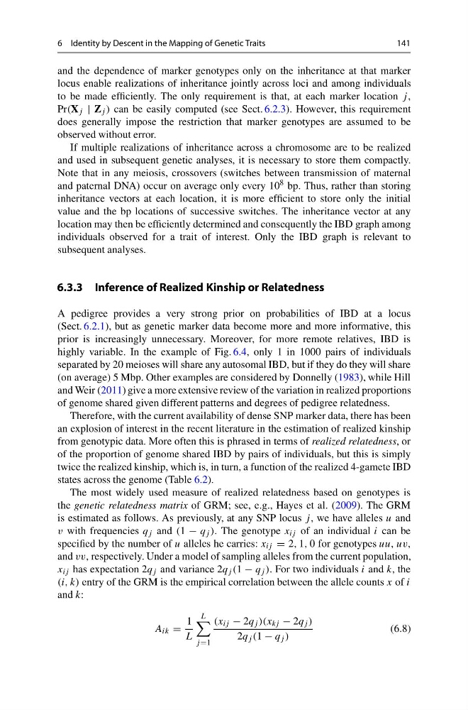
The most widely used measure of realized relatedness based on genotypes is
the genetic relatedness matrix of GRM; see, e.g., Hayes et al. (2009). The GRM
is estimated as follows. As previously, at any SNP locus j , we have alleles u and
v with frequencies q j and (1 − q j ). The genotype x ij of an individual i can be
specified by the number of u alleles he carries: x ij = 2, 1, 0 for genotypes uu, uv,
and vv, respectively. Under a model of sampling alleles from the current population,
x ij has expectation 2q j and variance 2q j (1 − q j ). For two individuals i and k, the
(i, k) entry of the GRM is the empirical correlation between the allele counts x of i
and k:
A ik =
1
L
L
j =1
(x ij − 2q j )(x kj − 2q j )
2q j (1 − q j )
(6.8)
141
and the dependence of marker genotypes only on the inheritance at that marker
locus enable realizations of inheritance jointly across loci and among individuals
to be made efficiently. The only requirement is that, at each marker location j ,
Pr(X j | Z j ) can be easily computed (see Sect. 6.2.3). However, this requirement
does generally impose the restriction that marker genotypes are assumed to be
observed without error.
If multiple realizations of inheritance across a chromosome are to be realized
and used in subsequent genetic analyses, it is necessary to store them compactly.
Note that in any meiosis, crossovers (switches between transmission of maternal
and paternal DNA) occur on average only every 10 8 bp. Thus, rather than storing
inheritance vectors at each location, it is more efficient to store only the initial
value and the bp locations of successive switches. The inheritance vector at any
location may then be efficiently determined and consequently the IBD graph among
individuals observed for a trait of interest. Only the IBD graph is relevant to
subsequent analyses.
6.3.3 Inference of Realized Kinship or Relatedness
A pedigree provides a very strong prior on probabilities of IBD at a locus
(Sect. 6.2.1), but as genetic marker data become more and more informative, this
prior is increasingly unnecessary. Moreover, for more remote relatives, IBD is
highly variable. In the example of Fig. 6.4, only 1 in 1000 pairs of individuals
separated by 20 meioses will share any autosomal IBD, but if they do they will share
(on average) 5 Mbp. Other examples are considered by Donnelly (1983), while Hill
and Weir (2011) give a more extensive review of the variation in realized proportions
of genome shared given different patterns and degrees of pedigree relatedness.
Therefore, with the current availability of dense SNP marker data, there has been
an explosion of interest in the recent literature in the estimation of realized kinship
from genotypic data. More often this is phrased in terms of realized relatedness, or
of the proportion of genome shared IBD by pairs of individuals, but this is simply
twice the realized kinship, which is, in turn, a function of the realized 4-gamete IBD
states across the genome (Table 6.2).
The most widely used measure of realized relatedness based on genotypes is
the genetic relatedness matrix of GRM; see, e.g., Hayes et al. (2009). The GRM
is estimated as follows. As previously, at any SNP locus j , we have alleles u and
v with frequencies q j and (1 − q j ). The genotype x ij of an individual i can be
specified by the number of u alleles he carries: x ij = 2, 1, 0 for genotypes uu, uv,
and vv, respectively. Under a model of sampling alleles from the current population,
x ij has expectation 2q j and variance 2q j (1 − q j ). For two individuals i and k, the
(i, k) entry of the GRM is the empirical correlation between the allele counts x of i
and k:
A ik =
1
L
L
j =1
(x ij − 2q j )(x kj − 2q j )
2q j (1 − q j )
(6.8)