

are obtained from push to push, it is advisable to check carefully
for artifacts (see Note 8).
6. Use Eq. 2 for the first attempt at curve fitting. Studies of simple
bimolecular reactions performed under pseudo-first-order
conditions should yield single exponential transients for
which Eq. 2 gives the observed rate (k obs ). Eq. 2 can also be
used to analyze fluorescence anisotropy data if there is no
change in fluorescence intensity accompanying the reaction
(see Note 7).
7. Extend the study to higher values of [X tot ] while keeping the
concentration of the other component unchanged. Although
the largest possible concentration range should be studied this
is not always possible. The largest usable value of [X tot ] will
depend upon the values of the individual rate constants. Thus,
for example, with an association rate constant (k 1 ) of the order
of 10
7 M
À1 s
À1 and an instrument dead time of 2 ms, the
largest value would be of the order of 50 μM
((k obs ¼ k +1 [X tot ] + k À1 ) > 500 s
À1 ) but would be significantly
lower if k À1 is large.
8. Inspect average and fit traces for each concentration measured.
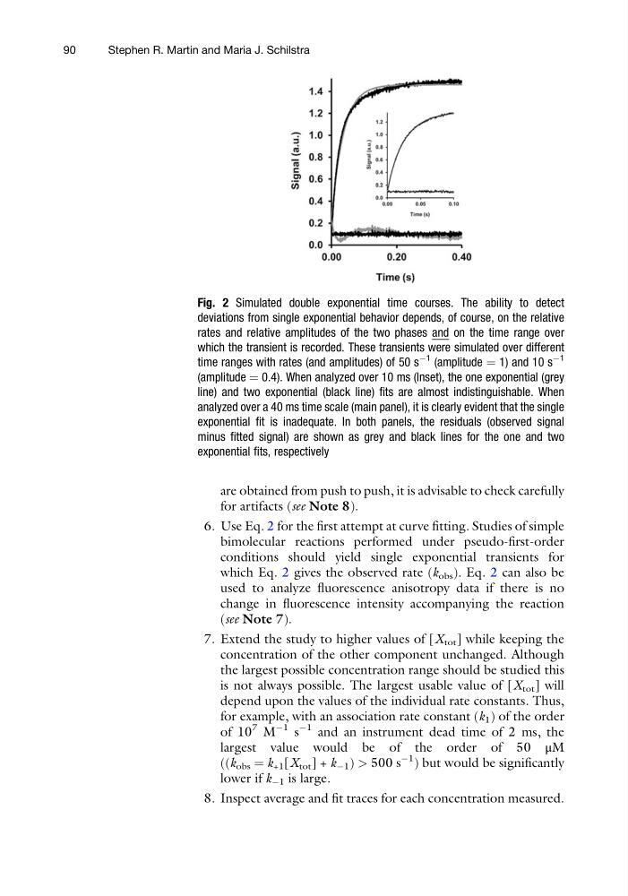
Fig. 2 Simulated double exponential time courses. The ability to detect
deviations from single exponential behavior depends, of course, on the relative
rates and relative amplitudes of the two phases and on the time range over
which the transient is recorded. These transients were simulated over different
time ranges with rates (and amplitudes) of 50 s
À1
(amplitude ¼ 1) and 10 s
À1
(amplitude ¼ 0.4). When analyzed over 10 ms (Inset), the one exponential (grey
line) and two exponential (black line) fits are almost indistinguishable. When
analyzed over a 40 ms time scale (main panel), it is clearly evident that the single
exponential fit is inadequate. In both panels, the residuals (observed signal
minus fitted signal) are shown as grey and black lines for the one and two
exponential fits, respectively
90
Stephen R. Martin and Maria J. Schilstra
for artifacts (see Note 8).
6. Use Eq. 2 for the first attempt at curve fitting. Studies of simple
bimolecular reactions performed under pseudo-first-order
conditions should yield single exponential transients for
which Eq. 2 gives the observed rate (k obs ). Eq. 2 can also be
used to analyze fluorescence anisotropy data if there is no
change in fluorescence intensity accompanying the reaction
(see Note 7).
7. Extend the study to higher values of [X tot ] while keeping the
concentration of the other component unchanged. Although
the largest possible concentration range should be studied this
is not always possible. The largest usable value of [X tot ] will
depend upon the values of the individual rate constants. Thus,
for example, with an association rate constant (k 1 ) of the order
of 10
7 M
À1 s
À1 and an instrument dead time of 2 ms, the
largest value would be of the order of 50 μM
((k obs ¼ k +1 [X tot ] + k À1 ) > 500 s
À1 ) but would be significantly
lower if k À1 is large.
8. Inspect average and fit traces for each concentration measured.
Fig. 2 Simulated double exponential time courses. The ability to detect
deviations from single exponential behavior depends, of course, on the relative
rates and relative amplitudes of the two phases and on the time range over
which the transient is recorded. These transients were simulated over different
time ranges with rates (and amplitudes) of 50 s
À1
(amplitude ¼ 1) and 10 s
À1
(amplitude ¼ 0.4). When analyzed over 10 ms (Inset), the one exponential (grey
line) and two exponential (black line) fits are almost indistinguishable. When
analyzed over a 40 ms time scale (main panel), it is clearly evident that the single
exponential fit is inadequate. In both panels, the residuals (observed signal
minus fitted signal) are shown as grey and black lines for the one and two
exponential fits, respectively
90
Stephen R. Martin and Maria J. Schilstra