

To analyze data:
7. Plot the fluorescence signal versus time for all ATP concentrations (see Fig. 4a, for example, data for the experiment in the
absence of DNA). Determine the initial rate of fluorescence
change (V F ¼ ΔF/Δt) at each ATP concentration by linear
regression using a data range where the fluorescence increase
is linear (boxed region in Fig. 4a) (see Note 10).
8. Correct the rate of fluorescence change V F for background by
subtracting the value at zero ATP.
9. Calculate the initial rate V using the corrected V F and the slope
from the calibration above (Eq. 3)
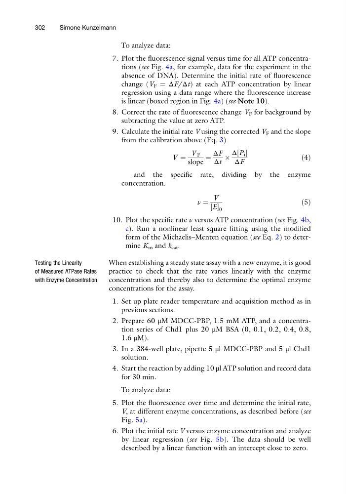
V ¼
V F
slope
¼
ΔF
Δt
Â
Δ P i
½
ΔF
ð4Þ
and the specific rate, dividing by the enzyme
concentration.
ν ¼
V
E
½ 0
ð5Þ
10. Plot the specific rate ν versus ATP concentration (see Fig. 4b,
c). Run a nonlinear least-square fitting using the modified
form of the Michaelis–Menten equation (see Eq. 2) to determine K m and k cat .
Testing the Linearity
of Measured ATPase Rates
with Enzyme Concentration
When establishing a steady state assay with a new enzyme, it is good
practice to check that the rate varies linearly with the enzyme
concentration and thereby also to determine the optimal enzyme
concentrations for the assay.
1. Set up plate reader temperature and acquisition method as in
previous sections.
2. Prepare 60 μM MDCC-PBP, 1.5 mM ATP, and a concentration series of Chd1 plus 20 μM BSA (0, 0.1, 0.2, 0.4, 0.8,
1.6 μM).
3. In a 384-well plate, pipette 5 μl MDCC-PBP and 5 μl Chd1
solution.
4. Start the reaction by adding 10 μl ATP solution and record data
for 30 min.
To analyze data:
5. Plot the fluorescence over time and determine the initial rate,
V, at different enzyme concentrations, as described before (see
Fig. 5a).
6. Plot the initial rate V versus enzyme concentration and analyze
by linear regression (see Fig. 5b). The data should be well
described by a linear function with an intercept close to zero.
302
Simone Kunzelmann
7. Plot the fluorescence signal versus time for all ATP concentrations (see Fig. 4a, for example, data for the experiment in the
absence of DNA). Determine the initial rate of fluorescence
change (V F ¼ ΔF/Δt) at each ATP concentration by linear
regression using a data range where the fluorescence increase
is linear (boxed region in Fig. 4a) (see Note 10).
8. Correct the rate of fluorescence change V F for background by
subtracting the value at zero ATP.
9. Calculate the initial rate V using the corrected V F and the slope
from the calibration above (Eq. 3)
V ¼
V F
slope
¼
ΔF
Δt
Â
Δ P i
½
ΔF
ð4Þ
and the specific rate, dividing by the enzyme
concentration.
ν ¼
V
E
½ 0
ð5Þ
10. Plot the specific rate ν versus ATP concentration (see Fig. 4b,
c). Run a nonlinear least-square fitting using the modified
form of the Michaelis–Menten equation (see Eq. 2) to determine K m and k cat .
Testing the Linearity
of Measured ATPase Rates
with Enzyme Concentration
When establishing a steady state assay with a new enzyme, it is good
practice to check that the rate varies linearly with the enzyme
concentration and thereby also to determine the optimal enzyme
concentrations for the assay.
1. Set up plate reader temperature and acquisition method as in
previous sections.
2. Prepare 60 μM MDCC-PBP, 1.5 mM ATP, and a concentration series of Chd1 plus 20 μM BSA (0, 0.1, 0.2, 0.4, 0.8,
1.6 μM).
3. In a 384-well plate, pipette 5 μl MDCC-PBP and 5 μl Chd1
solution.
4. Start the reaction by adding 10 μl ATP solution and record data
for 30 min.
To analyze data:
5. Plot the fluorescence over time and determine the initial rate,
V, at different enzyme concentrations, as described before (see
Fig. 5a).
6. Plot the initial rate V versus enzyme concentration and analyze
by linear regression (see Fig. 5b). The data should be well
described by a linear function with an intercept close to zero.
302
Simone Kunzelmann