

protein of similar molecular weight (30,000 Da compared to
22,000 Da for SBTI). Use the same incubation period, parameters, and style of capillaries to collect a data set as in steps 1
and 2 of this section, again naming the experiment
appropriately.
3.5 Data Analysis
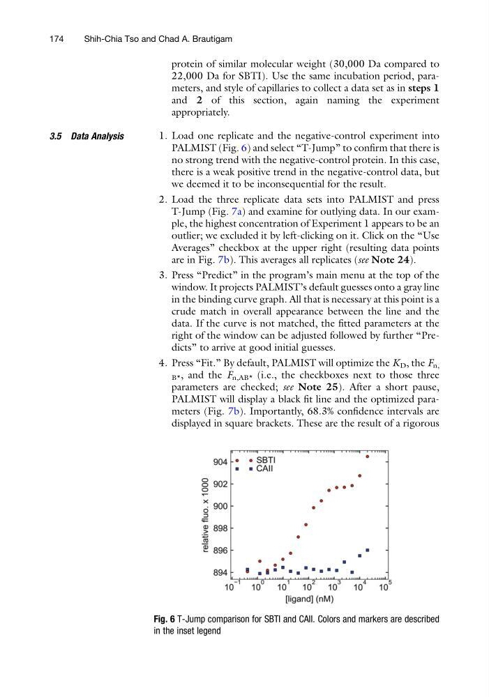
1. Load one replicate and the negative-control experiment into
PALMIST (Fig. 6) and select “T-Jump” to confirm that there is
no strong trend with the negative-control protein. In this case,
there is a weak positive trend in the negative-control data, but
we deemed it to be inconsequential for the result.
2. Load the three replicate data sets into PALMIST and press
T-Jump (Fig. 7a) and examine for outlying data. In our example, the highest concentration of Experiment 1 appears to be an
outlier; we excluded it by left-clicking on it. Click on the “Use
Averages” checkbox at the upper right (resulting data points
are in Fig. 7b). This averages all replicates (see Note 24).
3. Press “Predict” in the program’s main menu at the top of the
window. It projects PALMIST’s default guesses onto a gray line
in the binding curve graph. All that is necessary at this point is a
crude match in overall appearance between the line and the
data. If the curve is not matched, the fitted parameters at the
right of the window can be adjusted followed by further “Predicts” to arrive at good initial guesses.
4. Press “Fit.” By default, PALMIST will optimize the K D , the F n,
B* , and the F n,AB* (i.e., the checkboxes next to those three
parameters are checked; see Note 25). After a short pause,
PALMIST will display a black fit line and the optimized parameters (Fig. 7b). Importantly, 68.3% confidence intervals are
displayed in square brackets. These are the result of a rigorous
Fig. 6 T-Jump comparison for SBTI and CAII. Colors and markers are described
in the inset legend
174
Shih-Chia Tso and Chad A. Brautigam
22,000 Da for SBTI). Use the same incubation period, parameters, and style of capillaries to collect a data set as in steps 1
and 2 of this section, again naming the experiment
appropriately.
3.5 Data Analysis
1. Load one replicate and the negative-control experiment into
PALMIST (Fig. 6) and select “T-Jump” to confirm that there is
no strong trend with the negative-control protein. In this case,
there is a weak positive trend in the negative-control data, but
we deemed it to be inconsequential for the result.
2. Load the three replicate data sets into PALMIST and press
T-Jump (Fig. 7a) and examine for outlying data. In our example, the highest concentration of Experiment 1 appears to be an
outlier; we excluded it by left-clicking on it. Click on the “Use
Averages” checkbox at the upper right (resulting data points
are in Fig. 7b). This averages all replicates (see Note 24).
3. Press “Predict” in the program’s main menu at the top of the
window. It projects PALMIST’s default guesses onto a gray line
in the binding curve graph. All that is necessary at this point is a
crude match in overall appearance between the line and the
data. If the curve is not matched, the fitted parameters at the
right of the window can be adjusted followed by further “Predicts” to arrive at good initial guesses.
4. Press “Fit.” By default, PALMIST will optimize the K D , the F n,
B* , and the F n,AB* (i.e., the checkboxes next to those three
parameters are checked; see Note 25). After a short pause,
PALMIST will display a black fit line and the optimized parameters (Fig. 7b). Importantly, 68.3% confidence intervals are
displayed in square brackets. These are the result of a rigorous
Fig. 6 T-Jump comparison for SBTI and CAII. Colors and markers are described
in the inset legend
174
Shih-Chia Tso and Chad A. Brautigam