

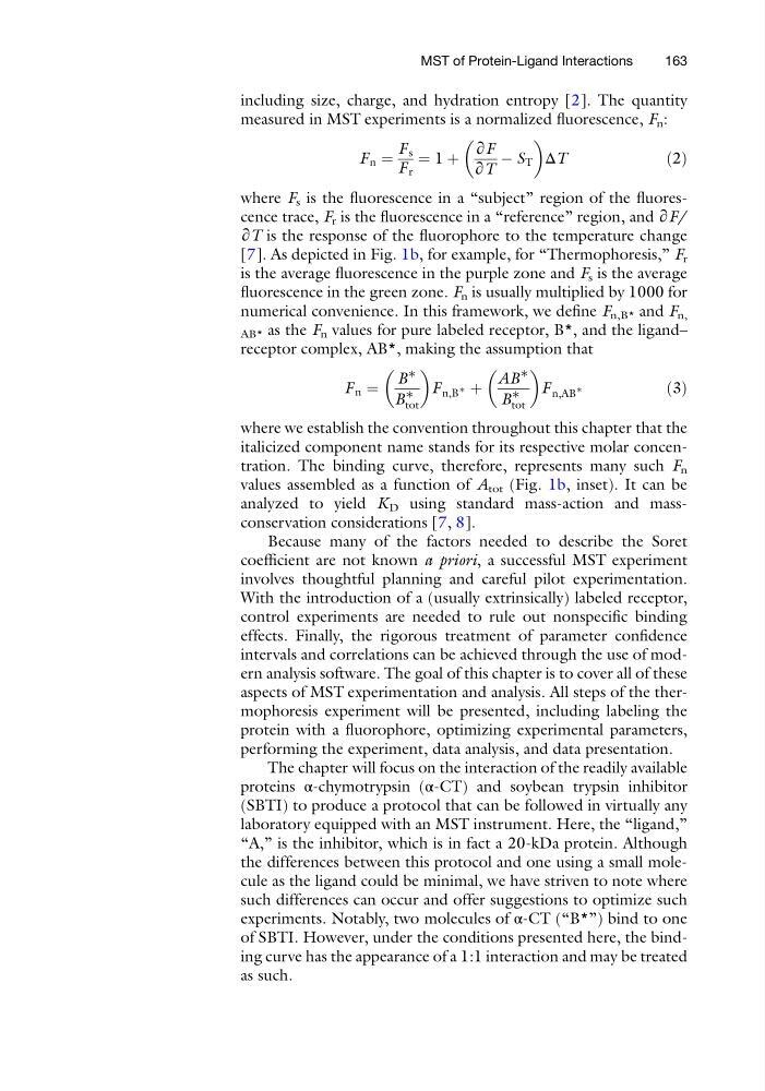
including size, charge, and hydration entropy [2]. The quantity
measured in MST experiments is a normalized fluorescence, F n :
F n ¼
F s
F r
¼ 1 þ
∂F
∂T
À S T
ΔT
ð2Þ
where F s is the fluorescence in a “subject” region of the fluorescence trace, F r is the fluorescence in a “reference” region, and ∂F/
∂T is the response of the fluorophore to the temperature change
[7]. As depicted in Fig. 1b, for example, for “Thermophoresis,” F r
is the average fluorescence in the purple zone and F s is the average
fluorescence in the green zone. F n is usually multiplied by 1000 for
numerical convenience. In this framework, we define F n,B* and F n,
AB* as the F n values for pure labeled receptor, B*, and the ligand–
receptor complex, AB*, making the assumption that
F n ¼
B
∗
B
∗
tot
F n,B
∗ þ
AB
∗
B
∗
tot
F n,AB
∗
ð3Þ
where we establish the convention throughout this chapter that the
italicized component name stands for its respective molar concentration. The binding curve, therefore, represents many such F n
values assembled as a function of A tot (Fig. 1b, inset). It can be
analyzed to yield K D using standard mass-action and massconservation considerations [7, 8].
Because many of the factors needed to describe the Soret
coefficient are not known a priori, a successful MST experiment
involves thoughtful planning and careful pilot experimentation.
With the introduction of a (usually extrinsically) labeled receptor,
control experiments are needed to rule out nonspecific binding
effects. Finally, the rigorous treatment of parameter confidence
intervals and correlations can be achieved through the use of modern analysis software. The goal of this chapter is to cover all of these
aspects of MST experimentation and analysis. All steps of the thermophoresis experiment will be presented, including labeling the
protein with a fluorophore, optimizing experimental parameters,
performing the experiment, data analysis, and data presentation.
The chapter will focus on the interaction of the readily available
proteins α-chymotrypsin (α-CT) and soybean trypsin inhibitor
(SBTI) to produce a protocol that can be followed in virtually any
laboratory equipped with an MST instrument. Here, the “ligand,”
“A,” is the inhibitor, which is in fact a 20-kDa protein. Although
the differences between this protocol and one using a small molecule as the ligand could be minimal, we have striven to note where
such differences can occur and offer suggestions to optimize such
experiments. Notably, two molecules of α-CT (“B*”) bind to one
of SBTI. However, under the conditions presented here, the binding curve has the appearance of a 1:1 interaction and may be treated
as such.
MST of Protein-Ligand Interactions
163
measured in MST experiments is a normalized fluorescence, F n :
F n ¼
F s
F r
¼ 1 þ
∂F
∂T
À S T
ΔT
ð2Þ
where F s is the fluorescence in a “subject” region of the fluorescence trace, F r is the fluorescence in a “reference” region, and ∂F/
∂T is the response of the fluorophore to the temperature change
[7]. As depicted in Fig. 1b, for example, for “Thermophoresis,” F r
is the average fluorescence in the purple zone and F s is the average
fluorescence in the green zone. F n is usually multiplied by 1000 for
numerical convenience. In this framework, we define F n,B* and F n,
AB* as the F n values for pure labeled receptor, B*, and the ligand–
receptor complex, AB*, making the assumption that
F n ¼
B
∗
B
∗
tot
F n,B
∗ þ
AB
∗
B
∗
tot
F n,AB
∗
ð3Þ
where we establish the convention throughout this chapter that the
italicized component name stands for its respective molar concentration. The binding curve, therefore, represents many such F n
values assembled as a function of A tot (Fig. 1b, inset). It can be
analyzed to yield K D using standard mass-action and massconservation considerations [7, 8].
Because many of the factors needed to describe the Soret
coefficient are not known a priori, a successful MST experiment
involves thoughtful planning and careful pilot experimentation.
With the introduction of a (usually extrinsically) labeled receptor,
control experiments are needed to rule out nonspecific binding
effects. Finally, the rigorous treatment of parameter confidence
intervals and correlations can be achieved through the use of modern analysis software. The goal of this chapter is to cover all of these
aspects of MST experimentation and analysis. All steps of the thermophoresis experiment will be presented, including labeling the
protein with a fluorophore, optimizing experimental parameters,
performing the experiment, data analysis, and data presentation.
The chapter will focus on the interaction of the readily available
proteins α-chymotrypsin (α-CT) and soybean trypsin inhibitor
(SBTI) to produce a protocol that can be followed in virtually any
laboratory equipped with an MST instrument. Here, the “ligand,”
“A,” is the inhibitor, which is in fact a 20-kDa protein. Although
the differences between this protocol and one using a small molecule as the ligand could be minimal, we have striven to note where
such differences can occur and offer suggestions to optimize such
experiments. Notably, two molecules of α-CT (“B*”) bind to one
of SBTI. However, under the conditions presented here, the binding curve has the appearance of a 1:1 interaction and may be treated
as such.
MST of Protein-Ligand Interactions
163