

d PL
∗
½
= dt ¼ k 2 PL
½ À k À2 PL
∗
½
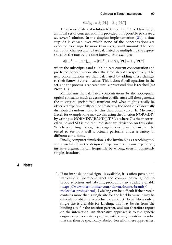
There is no analytical solution to this set of ODEs. However, if
an initial set of concentrations is provided, it is possible to create a
numerical solution. In the simplest implementation [21], a time
step Δt is chosen over which none of the concentrations are
expected to change by more than a very small amount. The concentration changes after dt are calculated by multiplying the expressions for the rate by the time interval. For example:
d PL
∗
½
¼ PL
∗
½
tþdt À PL
∗
½
t % dt k 2 PL
½ À k À2 PL
∗
½
ð
Þ
where the subscripts t and t + dt indicate current concentration and
predicted concentration after the time step dt, respectively. The
new concentrations are then calculated by adding these changes
to their (known) current values. This is done for all equations in the
set, and the process is repeated until a preset end time is reached (see
Note 15).
Multiplying the calculated concentrations by the appropriate
optical constants (such as extinction coefficients) will then generate
the theoretical (noise free) transient and what might actually be
observed experimentally can be created by the addition of normally
distributed random noise to this theoretical curve. In Microsoft
Excel, for example, one may do this using the function NORMINV
by writing ¼ NORMINV(RAND(),T,SD), where T is the theoretical value and SD is the required standard deviation on this value.
Whichever fitting package or program one is using can then be
tested to see how well it actually performs under a variety of
different conditions.
Finally, computer simulation is also invaluable as a teaching tool
and a useful aid in the design of experiments. In our experience,
intuitive arguments can frequently be wrong, even in apparently
simple situations.
4 Notes
1. If no intrinsic optical signal is available, it is often possible to
introduce a fluorescent label and comprehensive guides to
probe selection and labeling procedures are readily available
(https://www.thermofisher.com/uk/en/home/brands/
molecular-probes.html). Labeling can be difficult if the protein
contains more than a single site for the label because it may be
difficult to obtain a reproducible product. Even when only a
single site is available for labeling, this may be far from the
binding site for the reaction partner, and not therefore report
on the interaction. An alternative approach is to use genetic
engineering to create a protein with a single cysteine residue
that can then be specifically labeled. For all of these approaches,
Calmodulin Target Interactions
99
∗
½
= dt ¼ k 2 PL
½ À k À2 PL
∗
½
There is no analytical solution to this set of ODEs. However, if
an initial set of concentrations is provided, it is possible to create a
numerical solution. In the simplest implementation [21], a time
step Δt is chosen over which none of the concentrations are
expected to change by more than a very small amount. The concentration changes after dt are calculated by multiplying the expressions for the rate by the time interval. For example:
d PL
∗
½
¼ PL
∗
½
tþdt À PL
∗
½
t % dt k 2 PL
½ À k À2 PL
∗
½
ð
Þ
where the subscripts t and t + dt indicate current concentration and
predicted concentration after the time step dt, respectively. The
new concentrations are then calculated by adding these changes
to their (known) current values. This is done for all equations in the
set, and the process is repeated until a preset end time is reached (see
Note 15).
Multiplying the calculated concentrations by the appropriate
optical constants (such as extinction coefficients) will then generate
the theoretical (noise free) transient and what might actually be
observed experimentally can be created by the addition of normally
distributed random noise to this theoretical curve. In Microsoft
Excel, for example, one may do this using the function NORMINV
by writing ¼ NORMINV(RAND(),T,SD), where T is the theoretical value and SD is the required standard deviation on this value.
Whichever fitting package or program one is using can then be
tested to see how well it actually performs under a variety of
different conditions.
Finally, computer simulation is also invaluable as a teaching tool
and a useful aid in the design of experiments. In our experience,
intuitive arguments can frequently be wrong, even in apparently
simple situations.
4 Notes
1. If no intrinsic optical signal is available, it is often possible to
introduce a fluorescent label and comprehensive guides to
probe selection and labeling procedures are readily available
(https://www.thermofisher.com/uk/en/home/brands/
molecular-probes.html). Labeling can be difficult if the protein
contains more than a single site for the label because it may be
difficult to obtain a reproducible product. Even when only a
single site is available for labeling, this may be far from the
binding site for the reaction partner, and not therefore report
on the interaction. An alternative approach is to use genetic
engineering to create a protein with a single cysteine residue
that can then be specifically labeled. For all of these approaches,
Calmodulin Target Interactions
99