

flow methods. In this situation, the most commonly used approach
is to try to study the individual steps in isolation [16, 18, 19].
3.5 Data Analysis
and Simulation
In the preceding discussion, we have assumed that fitting the time
dependence of the observed signal to one or more exponential
terms will always be possible. However, the requirement for explicit
analytical solutions to the rate equations places severe constraints
on the experimental conditions that can be employed, and it will
not always be possible to work within these constraints. For example, if it is not possible to work under pseudo-first-order conditions,
it will be necessary to analyze progress curves using an iterative
method based on numerical integration of the appropriate differential rate equations [20].
Global analysis methods allow one to fit multiple kinetic data
sets obtained under different concentration conditions [17]. The
simultaneous analysis of the different data sets has the potential to
achieve better definition of the rate constants common to all the
sets. In favorable cases, it may allow the determination of kinetic
constants not obtainable by traditional methods and can be used to
distinguish between different kinetic models. Another strong point
of global analysis is that the different data sets can be obtained using
different methods, e.g., fluorescence intensity and anisotropy data,
in which the kinetic constants are nevertheless the same. In such
cases, it is important to weight the different data sets correctly. This
can be done by determining the standard deviation in the signal of a
reaction that has reached equilibrium. For example, using the last
5 ms of the transient shown in Fig. 2 would give a good estimate of
the standard deviation.
Having extracted rate constants by any of the methods
described here, it is almost always instructive to simulate the results
in order to see how well the data actually fits the assumed mechanism. This is most often done at the level of simulating how k obs
values depend upon the concentrations of the reagents. It can also
be very instructive to simulate individual reaction traces. This can
be done using any one of several freely available packages (http://
sbml.org/SBML_Software_Guide/SBML_Software_Summary)
that will simulate changes in concentrations with time. Although
many of these methods are very sophisticated, the principles are
relatively easy to understand and the simplest methods can be
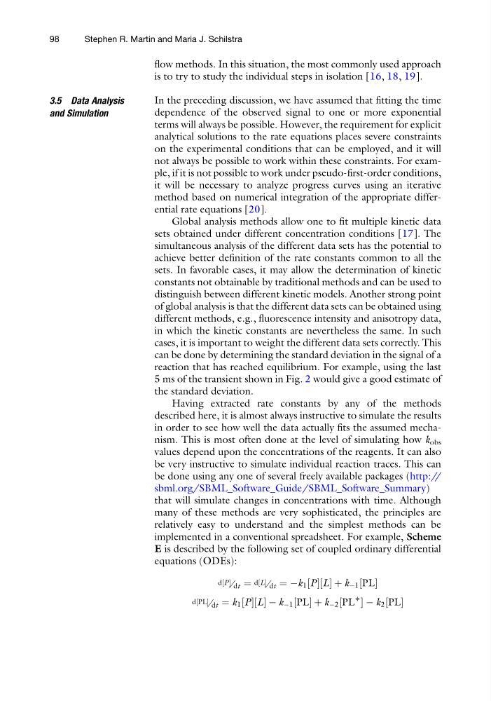
implemented in a conventional spreadsheet. For example, Scheme
E is described by the following set of coupled ordinary differential
equations (ODEs):
d P
½ = dt ¼ d L
½ = dt ¼ Àk 1 P
½ L
½ þ k À1 PL
½
d PL
½ = dt ¼ k 1 P
½ L
½ À k À1 PL
½ þ k À2 PL
∗
½
Àk 2 PL
½
98
Stephen R. Martin and Maria J. Schilstra
is to try to study the individual steps in isolation [16, 18, 19].
3.5 Data Analysis
and Simulation
In the preceding discussion, we have assumed that fitting the time
dependence of the observed signal to one or more exponential
terms will always be possible. However, the requirement for explicit
analytical solutions to the rate equations places severe constraints
on the experimental conditions that can be employed, and it will
not always be possible to work within these constraints. For example, if it is not possible to work under pseudo-first-order conditions,
it will be necessary to analyze progress curves using an iterative
method based on numerical integration of the appropriate differential rate equations [20].
Global analysis methods allow one to fit multiple kinetic data
sets obtained under different concentration conditions [17]. The
simultaneous analysis of the different data sets has the potential to
achieve better definition of the rate constants common to all the
sets. In favorable cases, it may allow the determination of kinetic
constants not obtainable by traditional methods and can be used to
distinguish between different kinetic models. Another strong point
of global analysis is that the different data sets can be obtained using
different methods, e.g., fluorescence intensity and anisotropy data,
in which the kinetic constants are nevertheless the same. In such
cases, it is important to weight the different data sets correctly. This
can be done by determining the standard deviation in the signal of a
reaction that has reached equilibrium. For example, using the last
5 ms of the transient shown in Fig. 2 would give a good estimate of
the standard deviation.
Having extracted rate constants by any of the methods
described here, it is almost always instructive to simulate the results
in order to see how well the data actually fits the assumed mechanism. This is most often done at the level of simulating how k obs
values depend upon the concentrations of the reagents. It can also
be very instructive to simulate individual reaction traces. This can
be done using any one of several freely available packages (http://
sbml.org/SBML_Software_Guide/SBML_Software_Summary)
that will simulate changes in concentrations with time. Although
many of these methods are very sophisticated, the principles are
relatively easy to understand and the simplest methods can be
implemented in a conventional spreadsheet. For example, Scheme
E is described by the following set of coupled ordinary differential
equations (ODEs):
d P
½ = dt ¼ d L
½ = dt ¼ Àk 1 P
½ L
½ þ k À1 PL
½
d PL
½ = dt ¼ k 1 P
½ L
½ À k À1 PL
½ þ k À2 PL
∗
½
Àk 2 PL
½
98
Stephen R. Martin and Maria J. Schilstra