

variables (Wakefield, 2013). The covariate, C i , was
mean centered to assist in the goodness-of-fit of the
model. The log of the relative risk of the fitted model
was established as log η i = β 0 + β 1 C i , where β 0 and
β 1 , expressed compactly as β are the parameters to
be estimated. These parameters were assigned a prior
distribution of β i ∼ N (0, 1000) and C i ∼ N (0, 1). The
distribution of β i was non-informative in order to make
sure that the posterior distribution is dominated by the
likelihood so as to enhance objectivity in the simulation process. The simulations were carried out using
the Metropolis-Hasting algorithm of McMC.
3.3 INLA formulation for both models
It was very easy implementing INLA for both models. All that was needed was to establish a relationship
between the response variable and the covariates,
indicate the required data and then apply the INLA
function. This seems not to be the case for the
implementation of the McMC algorithms.
4 RESULTS AND DISCUSSION
4.1 Results in terms of accuracy
This section states the parameter estimates and other
relevant plots of the simple and generalized linear
models. The details are as follows:
4.1.1 Simple linear model
For the purposes of convergence diagnostics, the trace,
and autocorrelation plots of tau, τ, were ascertained.
They are as shown in Figure 1. The corresponding convergence diagnostics plots of β were similar to those
of τ so they were excluded to avoid tautology.
Figure 1. Trace and autocorrelation plots of the McMC
realizations of Tau, τ.
Secondly, a table showing the mean values of the
parameters estimated by the McMC and INLA techniques, with their respective standard deviations (in
brackets) and the true values of the parameters of
interest, is as shown in Table 1 above.
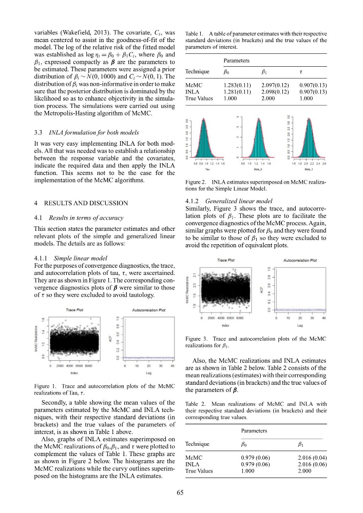
Also, graphs of INLA estimates superimposed on
the McMC realizations of β 0 ,β 1 , and τ were plotted to
complement the values of Table 1. These graphs are
as shown in Figure 2 below. The histograms are the
McMC realizations while the curvy outlines superimposed on the histograms are the INLA estimates.
Table 1. A table of parameter estimates with their respective
standard deviations (in brackets) and the true values of the
parameters of interest.
Parameters
Technique
β 0
β 1
τ
McMC
1.283(0.11)
2.097(0.12)
0.907(0.13)
INLA
1.281(0.11)
2.098(0.12)
0.907(0.13)
True Values
1.000
2.000
1.000
Figure 2. INLA estimates superimposed on McMC realizations for the Simple Linear Model.
4.1.2 Generalized linear model
Similarly, Figure 3 shows the trace, and autocorrelation plots of β 1 . These plots are to facilitate the
convergence diagnostics of the McMC process. Again,
similar graphs were plotted for β 0 and they were found
to be similar to those of β 1 so they were excluded to
avoid the repetition of equivalent plots.
Figure 3. Trace and autocorrelation plots of the McMC
realizations for β 1 .
Also, the McMC realizations and INLA estimates
are as shown in Table 2 below. Table 2 consists of the
mean realizations (estimates) with their corresponding
standard deviations (in brackets) and the true values of
the parameters of β.
Table 2. Mean realizations of McMC and INLA with
their respective standard deviations (in brackets) and their
corresponding true values.
Parameters
Technique
β 0
β 1
McMC
0.979 (0.06)
2.016 (0.04)
INLA
0.979 (0.06)
2.016 (0.06)
True Values
1.000
2.000
65
mean centered to assist in the goodness-of-fit of the
model. The log of the relative risk of the fitted model
was established as log η i = β 0 + β 1 C i , where β 0 and
β 1 , expressed compactly as β are the parameters to
be estimated. These parameters were assigned a prior
distribution of β i ∼ N (0, 1000) and C i ∼ N (0, 1). The
distribution of β i was non-informative in order to make
sure that the posterior distribution is dominated by the
likelihood so as to enhance objectivity in the simulation process. The simulations were carried out using
the Metropolis-Hasting algorithm of McMC.
3.3 INLA formulation for both models
It was very easy implementing INLA for both models. All that was needed was to establish a relationship
between the response variable and the covariates,
indicate the required data and then apply the INLA
function. This seems not to be the case for the
implementation of the McMC algorithms.
4 RESULTS AND DISCUSSION
4.1 Results in terms of accuracy
This section states the parameter estimates and other
relevant plots of the simple and generalized linear
models. The details are as follows:
4.1.1 Simple linear model
For the purposes of convergence diagnostics, the trace,
and autocorrelation plots of tau, τ, were ascertained.
They are as shown in Figure 1. The corresponding convergence diagnostics plots of β were similar to those
of τ so they were excluded to avoid tautology.
Figure 1. Trace and autocorrelation plots of the McMC
realizations of Tau, τ.
Secondly, a table showing the mean values of the
parameters estimated by the McMC and INLA techniques, with their respective standard deviations (in
brackets) and the true values of the parameters of
interest, is as shown in Table 1 above.
Also, graphs of INLA estimates superimposed on
the McMC realizations of β 0 ,β 1 , and τ were plotted to
complement the values of Table 1. These graphs are
as shown in Figure 2 below. The histograms are the
McMC realizations while the curvy outlines superimposed on the histograms are the INLA estimates.
Table 1. A table of parameter estimates with their respective
standard deviations (in brackets) and the true values of the
parameters of interest.
Parameters
Technique
β 0
β 1
τ
McMC
1.283(0.11)
2.097(0.12)
0.907(0.13)
INLA
1.281(0.11)
2.098(0.12)
0.907(0.13)
True Values
1.000
2.000
1.000
Figure 2. INLA estimates superimposed on McMC realizations for the Simple Linear Model.
4.1.2 Generalized linear model
Similarly, Figure 3 shows the trace, and autocorrelation plots of β 1 . These plots are to facilitate the
convergence diagnostics of the McMC process. Again,
similar graphs were plotted for β 0 and they were found
to be similar to those of β 1 so they were excluded to
avoid the repetition of equivalent plots.
Figure 3. Trace and autocorrelation plots of the McMC
realizations for β 1 .
Also, the McMC realizations and INLA estimates
are as shown in Table 2 below. Table 2 consists of the
mean realizations (estimates) with their corresponding
standard deviations (in brackets) and the true values of
the parameters of β.
Table 2. Mean realizations of McMC and INLA with
their respective standard deviations (in brackets) and their
corresponding true values.
Parameters
Technique
β 0
β 1
McMC
0.979 (0.06)
2.016 (0.04)
INLA
0.979 (0.06)
2.016 (0.06)
True Values
1.000
2.000
65