

4.3 The econometric model: vector error correction
model
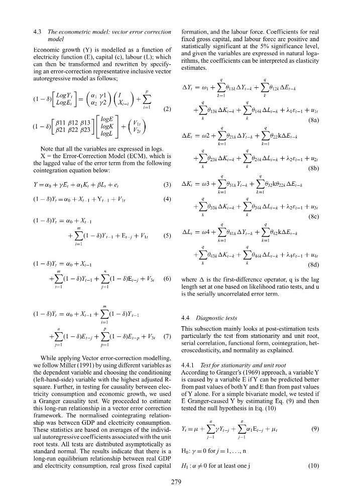
Economic growth (Y) is modelled as a function of
electricity function (E), capital (c), labour (L); which
can then be transformed and rewritten by specifying an error-correction representative inclusive vector
autoregressive model as follows;
(1 − δ)
LogY t
LogE t
=
α 1 γ1
α 2 γ2
I
X t−i
+
p
i=1
(2)
(1 − δ)
β11 β12 β13
β21 β22 β23
⎡
⎣
logE
logK
logL
⎤
⎦ +
V 1t
V 2t
Note that all the variables are expressed in logs.
X = the Error-Correction Model (ECM), which is
the lagged value of the error term from the following
cointegration equation below:
Y = α 0 + γE t + α 1 K t + βL t + e t
(3)
(1 − δ)Y t = α 0 + X t−1 + Y t−1 + V 1t
(4)
(1 − δ)Y t = α 0 + X t−1
+
m
i=1
(1 − δ)Y t−1 + E t−j + V 1t
(5)
(1 − δ)Y t = α 0 + X t−1
+
m
i=1
(1 − δ)Y t−1 +
n
j=1
(1 − δ)E t−j + V 3t (6)
(1 − δ)Y t = α 0 + X t−1 +
m
i=1
(1 − δ)Y t−1
+
n
j=1
(1 − δ)E t−j +
p
p=1
(1 − δ)E t−p + V 3t (7)
While applying Vector error-correction modelling,
we follow Miller (1991) by using different variables as
the dependent variable and choosing the conditioning
(left-hand-side) variable with the highest adjusted Rsquare. Further, in testing for causality between electricity consumption and economic growth, we used
a Granger causality test. We proceeded to estimate
this long-run relationship in a vector error correction
framework. The normalised cointegrating relationship was between GDP and electricity consumption.
These statistics are based on averages of the individual autoregressive coefficients associated with the unit
root tests. All tests are distributed asymptotically as
standard normal. The results indicate that there is a
long-run equilibrium relationship between real GDP
and electricity consumption, real gross fixed capital
formation, and the labour force. Coefficients for real
fixed gross capital, and labour force are positive and
statistically significant at the 5% significance level,
and given the variables are expressed in natural logarithms, the coefficients can be interpreted as elasticity
estimates.
Y t = ω 1 +
q
k=1
θ 11k Y t−k +
q
k
θ 12k E t−k
+
q
k
θ 13k K t−k +
q
k
θ 14k L t−k + λ 1 ε t−1 + u 1t
(8a)
E t = ω2 +
q
k=1
θ 21k Y t−k +
q
k=1
θ 22 kE t−k
+
q
k
θ 23k K t−k +
q
k
θ 24k L t−k + λ 2 ε t−1 + u 2t
(8b)
K t = ω3 +
q
k=1
θ 31k Y t−k +
q
k=1
θ 32 kθ 22k E t−k
+
q
k
θ 33k K t−k +
q
k
θ 34k L t−k + λ 2 ε t−1 + u 3t
(8c)
L t = ω4 +
q
k=1
θ 41k Y t−k +
q
k=1
θ 42 kE t−k
+
q
k
θ 43k K t−k +
q
k
θ 44k L t−k + λ 4 ε t−1 + u 4t
(8d)
where is the first-difference operator, q is the lag
length set at one based on likelihood ratio tests, and u
is the serially uncorrelated error term.
4.4 Diagnostic tests
This subsection mainly looks at post-estimation tests
particularly the test from stationarity and unit root,
serial correlation, functional form, cointegration, heteroscedasticity, and normality as explained.
4.4.1 Test for stationarity and unit root
According to Granger’s (1969) approach, a variable Y
is caused by a variable E if Y can be predicted better
from past values of both Y and E than from past values
of Y alone. For a simple bivariate model, we tested if
E Granger-caused Y by estimating Eq. (9) and then
tested the null hypothesis in Eq. (10)
Y t = µ +
n
j−1
γY t−j +
n
j−1
α 1 E t−j + µ t
(9)
H 0 : γ = 0 for j = 1, . . ., n
H 1 : α = 0 for at least one j
(10)
279
model
Economic growth (Y) is modelled as a function of
electricity function (E), capital (c), labour (L); which
can then be transformed and rewritten by specifying an error-correction representative inclusive vector
autoregressive model as follows;
(1 − δ)
LogY t
LogE t
=
α 1 γ1
α 2 γ2
I
X t−i
+
p
i=1
(2)
(1 − δ)
β11 β12 β13
β21 β22 β23
⎡
⎣
logE
logK
logL
⎤
⎦ +
V 1t
V 2t
Note that all the variables are expressed in logs.
X = the Error-Correction Model (ECM), which is
the lagged value of the error term from the following
cointegration equation below:
Y = α 0 + γE t + α 1 K t + βL t + e t
(3)
(1 − δ)Y t = α 0 + X t−1 + Y t−1 + V 1t
(4)
(1 − δ)Y t = α 0 + X t−1
+
m
i=1
(1 − δ)Y t−1 + E t−j + V 1t
(5)
(1 − δ)Y t = α 0 + X t−1
+
m
i=1
(1 − δ)Y t−1 +
n
j=1
(1 − δ)E t−j + V 3t (6)
(1 − δ)Y t = α 0 + X t−1 +
m
i=1
(1 − δ)Y t−1
+
n
j=1
(1 − δ)E t−j +
p
p=1
(1 − δ)E t−p + V 3t (7)
While applying Vector error-correction modelling,
we follow Miller (1991) by using different variables as
the dependent variable and choosing the conditioning
(left-hand-side) variable with the highest adjusted Rsquare. Further, in testing for causality between electricity consumption and economic growth, we used
a Granger causality test. We proceeded to estimate
this long-run relationship in a vector error correction
framework. The normalised cointegrating relationship was between GDP and electricity consumption.
These statistics are based on averages of the individual autoregressive coefficients associated with the unit
root tests. All tests are distributed asymptotically as
standard normal. The results indicate that there is a
long-run equilibrium relationship between real GDP
and electricity consumption, real gross fixed capital
formation, and the labour force. Coefficients for real
fixed gross capital, and labour force are positive and
statistically significant at the 5% significance level,
and given the variables are expressed in natural logarithms, the coefficients can be interpreted as elasticity
estimates.
Y t = ω 1 +
q
k=1
θ 11k Y t−k +
q
k
θ 12k E t−k
+
q
k
θ 13k K t−k +
q
k
θ 14k L t−k + λ 1 ε t−1 + u 1t
(8a)
E t = ω2 +
q
k=1
θ 21k Y t−k +
q
k=1
θ 22 kE t−k
+
q
k
θ 23k K t−k +
q
k
θ 24k L t−k + λ 2 ε t−1 + u 2t
(8b)
K t = ω3 +
q
k=1
θ 31k Y t−k +
q
k=1
θ 32 kθ 22k E t−k
+
q
k
θ 33k K t−k +
q
k
θ 34k L t−k + λ 2 ε t−1 + u 3t
(8c)
L t = ω4 +
q
k=1
θ 41k Y t−k +
q
k=1
θ 42 kE t−k
+
q
k
θ 43k K t−k +
q
k
θ 44k L t−k + λ 4 ε t−1 + u 4t
(8d)
where is the first-difference operator, q is the lag
length set at one based on likelihood ratio tests, and u
is the serially uncorrelated error term.
4.4 Diagnostic tests
This subsection mainly looks at post-estimation tests
particularly the test from stationarity and unit root,
serial correlation, functional form, cointegration, heteroscedasticity, and normality as explained.
4.4.1 Test for stationarity and unit root
According to Granger’s (1969) approach, a variable Y
is caused by a variable E if Y can be predicted better
from past values of both Y and E than from past values
of Y alone. For a simple bivariate model, we tested if
E Granger-caused Y by estimating Eq. (9) and then
tested the null hypothesis in Eq. (10)
Y t = µ +
n
j−1
γY t−j +
n
j−1
α 1 E t−j + µ t
(9)
H 0 : γ = 0 for j = 1, . . ., n
H 1 : α = 0 for at least one j
(10)
279