

uses separate simulations of the unbound peptide is also described.
The free energy function uses implicit solvent, which includes a
Poisson–Boltzmann electrostatic term plus a Surface Area (SA) and
a van der Waals (vdW) term. Taking the free energy difference
between the bound and unbound structures and averaging over
all the snapshots we obtain a binding free energy. Obviously, some
free energy components are not accounted for, such as translational
entropy. But they are expected to cancel out when we compare
several peptide (or protein) variants. The free energy function
requires some parameterization and testing before it can be applied.
Here, we outline the method, its parameterization using experimental binding free energies and its application to designed Sdc1
sequences. The method is also schematized in Fig. 3.
3.1 Explicit-Solvent
MD to Characterize
PDZ–Peptide
Complexes
MD is done with explicit solvent and only a few restraints on the
complex. Thus, the fixed backbone approximation from the CPD
stage is removed. Simulations lengths of 50–100 ns are used, which
allows the free energy function to converge. It also gives time for
the backbone to rearrange, if necessary. If, for a predicted variant,
the backbone rearranges significantly and/or the peptide starts to
detach, it suggests the particular complex is unstable and may
invalidate the CPD prediction.
Adaptive MC
Experimental
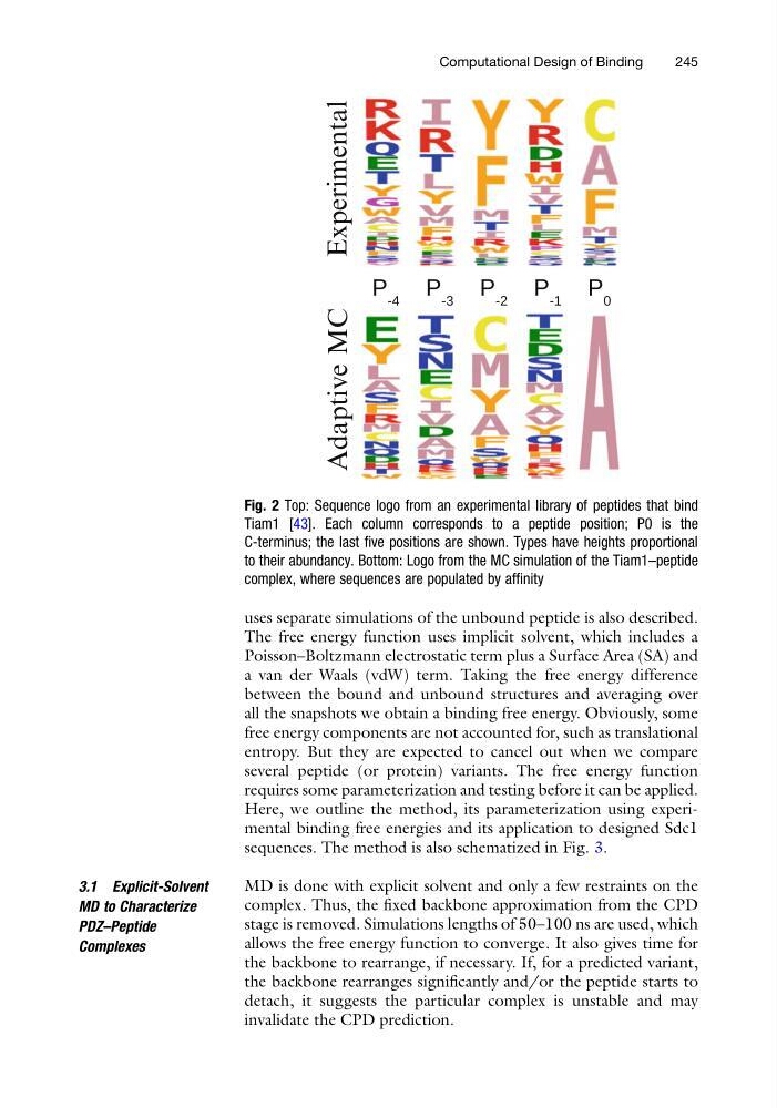
Fig. 2 Top: Sequence logo from an experimental library of peptides that bind
Tiam1 [43]. Each column corresponds to a peptide position; P0 is the
C-terminus; the last five positions are shown. Types have heights proportional
to their abundancy. Bottom: Logo from the MC simulation of the Tiam1–peptide
complex, where sequences are populated by affinity
Computational Design of Binding
245
The free energy function uses implicit solvent, which includes a
Poisson–Boltzmann electrostatic term plus a Surface Area (SA) and
a van der Waals (vdW) term. Taking the free energy difference
between the bound and unbound structures and averaging over
all the snapshots we obtain a binding free energy. Obviously, some
free energy components are not accounted for, such as translational
entropy. But they are expected to cancel out when we compare
several peptide (or protein) variants. The free energy function
requires some parameterization and testing before it can be applied.
Here, we outline the method, its parameterization using experimental binding free energies and its application to designed Sdc1
sequences. The method is also schematized in Fig. 3.
3.1 Explicit-Solvent
MD to Characterize
PDZ–Peptide
Complexes
MD is done with explicit solvent and only a few restraints on the
complex. Thus, the fixed backbone approximation from the CPD
stage is removed. Simulations lengths of 50–100 ns are used, which
allows the free energy function to converge. It also gives time for
the backbone to rearrange, if necessary. If, for a predicted variant,
the backbone rearranges significantly and/or the peptide starts to
detach, it suggests the particular complex is unstable and may
invalidate the CPD prediction.
Adaptive MC
Experimental
Fig. 2 Top: Sequence logo from an experimental library of peptides that bind
Tiam1 [43]. Each column corresponds to a peptide position; P0 is the
C-terminus; the last five positions are shown. Types have heights proportional
to their abundancy. Bottom: Logo from the MC simulation of the Tiam1–peptide
complex, where sequences are populated by affinity
Computational Design of Binding
245