

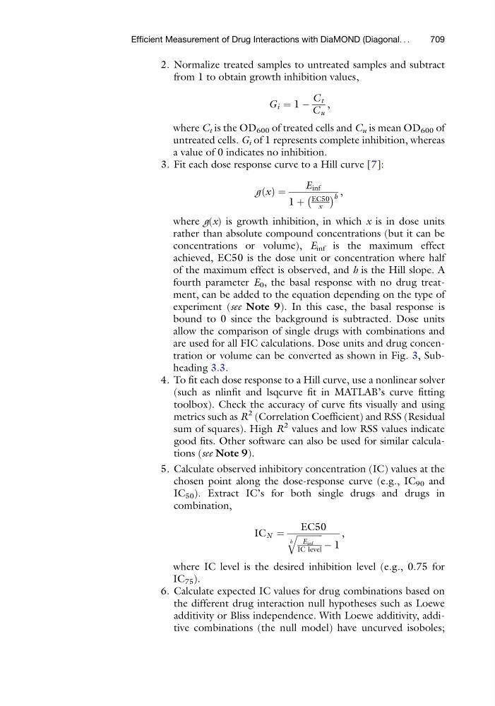
2. Normalize treated samples to untreated samples and subtract
from 1 to obtain growth inhibition values,
G i ¼ 1 À
C t
C u
,
where C t is the OD 600 of treated cells and C u is mean OD 600 of
untreated cells. G i of 1 represents complete inhibition, whereas
a value of 0 indicates no inhibition.
3. Fit each dose response curve to a Hill curve [7]:
g x
ð Þ ¼
E inf
1 þ
EC50
x
À
Á h ,
where g(x) is growth inhibition, in which x is in dose units
rather than absolute compound concentrations (but it can be
concentrations or volume), E inf is the maximum effect
achieved, EC50 is the dose unit or concentration where half
of the maximum effect is observed, and h is the Hill slope. A
fourth parameter E 0 , the basal response with no drug treatment, can be added to the equation depending on the type of
experiment (see Note 9). In this case, the basal response is
bound to 0 since the background is subtracted. Dose units
allow the comparison of single drugs with combinations and
are used for all FIC calculations. Dose units and drug concentration or volume can be converted as shown in Fig. 3, Subheading 3.3.
4. To fit each dose response to a Hill curve, use a nonlinear solver
(such as nlinfit and lsqcurve fit in MATLAB’s curve fitting
toolbox). Check the accuracy of curve fits visually and using
metrics such as R
2 (Correlation Coefficient) and RSS (Residual
sum of squares). High R
2 values and low RSS values indicate
good fits. Other software can also be used for similar calculations (see Note 9).
5. Calculate observed inhibitory concentration (IC) values at the
chosen point along the dose-response curve (e.g., IC 90 and
IC 50 ). Extract IC’s for both single drugs and drugs in
combination,
IC N ¼
EC50
ffiffiffiffiffiffiffiffiffiffiffi ffi
E inf
IC level
h
q
À 1
,
where IC level is the desired inhibition level (e.g., 0.75 for
IC 75 ).
6. Calculate expected IC values for drug combinations based on
the different drug interaction null hypotheses such as Loewe
additivity or Bliss independence. With Loewe additivity, additive combinations (the null model) have uncurved isoboles;
Efficient Measurement of Drug Interactions with DiaMOND (Diagonal. . .
709