

Processes 2019, 7, 163
It is not guaranteed that a turning point bifurcation will be reached. Pitchfork and transcritical
bifurcations could also result.
2.1.2. Optimization for Oscillatory Systems
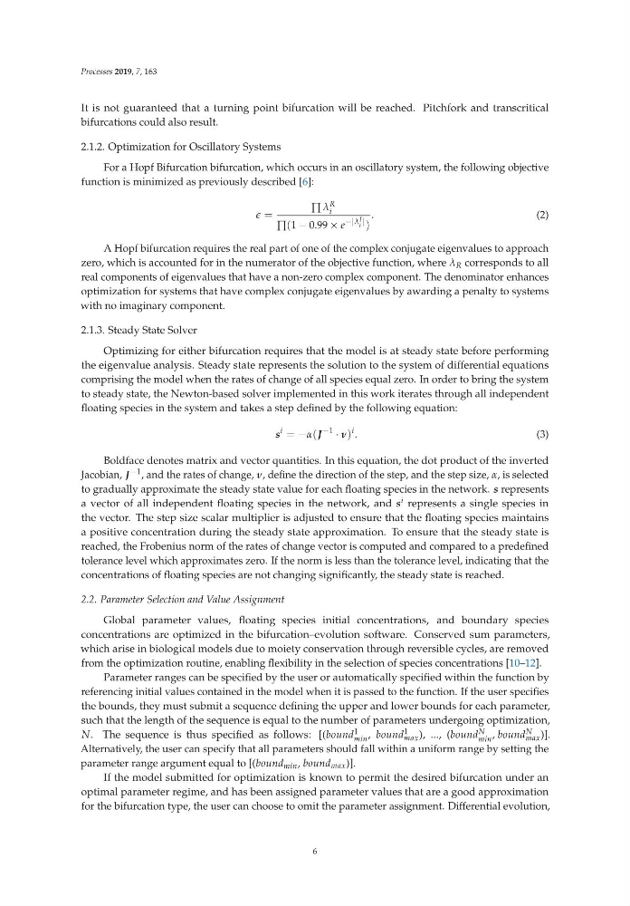
For a Hopf Bifurcation bifurcation, which occurs in an oscillatory system, the following objective
function is minimized as previously described [6]:
ǫ =
∏ λ R
i
∏(1 − 0.99 × e
−|λ I
i | )
.
(2)
A Hopf bifurcation requires the real part of one of the complex conjugate eigenvalues to approach
zero, which is accounted for in the numerator of the objective function, where λ R corresponds to all
real components of eigenvalues that have a non-zero complex component. The denominator enhances
optimization for systems that have complex conjugate eigenvalues by awarding a penalty to systems
with no imaginary component.
2.1.3. Steady State Solver
Optimizing for either bifurcation requires that the model is at steady state before performing
the eigenvalue analysis. Steady state represents the solution to the system of differential equations
comprising the model when the rates of change of all species equal zero. In order to bring the system
to steady state, the Newton-based solver implemented in this work iterates through all independent
floating species in the system and takes a step defined by the following equation:
s
i = −α(J
−1 · ν)
i .
(3)
Boldface denotes matrix and vector quantities. In this equation, the dot product of the inverted
Jacobian, J −1 , and the rates of change, ν, define the direction of the step, and the step size, α, is selected
to gradually approximate the steady state value for each floating species in the network. s represents
a vector of all independent floating species in the network, and s i represents a single species in
the vector. The step size scalar multiplier is adjusted to ensure that the floating species maintains
a positive concentration during the steady state approximation. To ensure that the steady state is
reached, the Frobenius norm of the rates of change vector is computed and compared to a predefined
tolerance level which approximates zero. If the norm is less than the tolerance level, indicating that the
concentrations of floating species are not changing significantly, the steady state is reached.
2.2. Parameter Selection and Value Assignment
Global parameter values, floating species initial concentrations, and boundary species
concentrations are optimized in the bifurcation–evolution software. Conserved sum parameters,
which arise in biological models due to moiety conservation through reversible cycles, are removed
from the optimization routine, enabling flexibility in the selection of species concentrations [10–12].
Parameter ranges can be specified by the user or automatically specified within the function by
referencing initial values contained in the model when it is passed to the function. If the user specifies
the bounds, they must submit a sequence defining the upper and lower bounds for each parameter,
such that the length of the sequence is equal to the number of parameters undergoing optimization,
N. The sequence is thus specified as follows: [(bound 1
min , bound 1
max ), ..., (bound N
min , bound N
max )].
Alternatively, the user can specify that all parameters should fall within a uniform range by setting the
parameter range argument equal to [(bound min , bound max )].
If the model submitted for optimization is known to permit the desired bifurcation under an
optimal parameter regime, and has been assigned parameter values that are a good approximation
for the bifurcation type, the user can choose to omit the parameter assignment. Differential evolution,
6
It is not guaranteed that a turning point bifurcation will be reached. Pitchfork and transcritical
bifurcations could also result.
2.1.2. Optimization for Oscillatory Systems
For a Hopf Bifurcation bifurcation, which occurs in an oscillatory system, the following objective
function is minimized as previously described [6]:
ǫ =
∏ λ R
i
∏(1 − 0.99 × e
−|λ I
i | )
.
(2)
A Hopf bifurcation requires the real part of one of the complex conjugate eigenvalues to approach
zero, which is accounted for in the numerator of the objective function, where λ R corresponds to all
real components of eigenvalues that have a non-zero complex component. The denominator enhances
optimization for systems that have complex conjugate eigenvalues by awarding a penalty to systems
with no imaginary component.
2.1.3. Steady State Solver
Optimizing for either bifurcation requires that the model is at steady state before performing
the eigenvalue analysis. Steady state represents the solution to the system of differential equations
comprising the model when the rates of change of all species equal zero. In order to bring the system
to steady state, the Newton-based solver implemented in this work iterates through all independent
floating species in the system and takes a step defined by the following equation:
s
i = −α(J
−1 · ν)
i .
(3)
Boldface denotes matrix and vector quantities. In this equation, the dot product of the inverted
Jacobian, J −1 , and the rates of change, ν, define the direction of the step, and the step size, α, is selected
to gradually approximate the steady state value for each floating species in the network. s represents
a vector of all independent floating species in the network, and s i represents a single species in
the vector. The step size scalar multiplier is adjusted to ensure that the floating species maintains
a positive concentration during the steady state approximation. To ensure that the steady state is
reached, the Frobenius norm of the rates of change vector is computed and compared to a predefined
tolerance level which approximates zero. If the norm is less than the tolerance level, indicating that the
concentrations of floating species are not changing significantly, the steady state is reached.
2.2. Parameter Selection and Value Assignment
Global parameter values, floating species initial concentrations, and boundary species
concentrations are optimized in the bifurcation–evolution software. Conserved sum parameters,
which arise in biological models due to moiety conservation through reversible cycles, are removed
from the optimization routine, enabling flexibility in the selection of species concentrations [10–12].
Parameter ranges can be specified by the user or automatically specified within the function by
referencing initial values contained in the model when it is passed to the function. If the user specifies
the bounds, they must submit a sequence defining the upper and lower bounds for each parameter,
such that the length of the sequence is equal to the number of parameters undergoing optimization,
N. The sequence is thus specified as follows: [(bound 1
min , bound 1
max ), ..., (bound N
min , bound N
max )].
Alternatively, the user can specify that all parameters should fall within a uniform range by setting the
parameter range argument equal to [(bound min , bound max )].
If the model submitted for optimization is known to permit the desired bifurcation under an
optimal parameter regime, and has been assigned parameter values that are a good approximation
for the bifurcation type, the user can choose to omit the parameter assignment. Differential evolution,
6