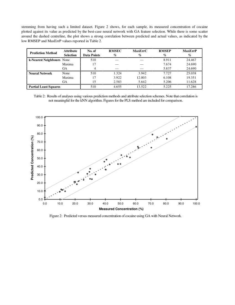
stemming from having such a limited dataset. Figure 2 shows, for each sample, its measured concentration of cocaine
plotted against its value as predicted by the best-case neural network with GA feature selection. While there is some scatter
around the dashed centreline, the plot shows a strong correlation between predicted and actual values, as indicated by the
low RMSEP and MaxErrP values reported in Table 2.
Prediction Method
Attribute
Selection
No. of
Data Points
RMSEC
%
MaxErrC
%
RMSEP
%
MaxErrP
%
k-Nearest Neighbours None
510
—
—
8.911
24.467
Maxima
17
—
—
7.674
24.690
GA
4
—
—
5.837
24.690
Neural Network
None
510
1.324
3.942
7.727
25.038
Maxima
17
3.922
12.003
6.108
19.351
GA
15
2.583
5.642
5.206
11.628
Partial Least Squares
510
4.655
13.522
5.225
17.286
Table 2: Results of analyses using various prediction methods and attribute selection schemes. Note that correlation is
not meaningful for the kNN algorithm. Figures for the PLS method are included for comparison.
0.0
10.0
20.0
30.0
40.0
50.0
60.0
70.0
80.0
90.0
100.0
0.0
10.0
20.0
30.0
40.0
50.0
60.0
70.0
80.0
90.0
100.0
Measured Concentration (%)
Predicted Concentration (%)
Figure 2: Predicted versus measured concentration of cocaine using GA with Neural Network.