

20
A. G. RYDER
0
2
4
6
8
10
12
14
16
18
20
40
60
80
100
y = a(exp(bx)),
std-err:2.62
max dev:6.60,
r
2
=0.65
a=0.197, b=0.0456
(B)
Alkane conc. (%w/w, corr.)
Average lifetime, ns.
0
2
4
6
8
10
12
14
16
18
40
60
80
100
(C)
y = a(exp(bx)),
std-err:2.47
max dev:7.16,
r
2
=0.69
a=0.0356, b=0.0603
Alkane & Losses % (w/w )
Average lifetime, ns
0
2
4
6
8
10
12
14
16
18
10
30
50
70
(A)
Alkane conc. (%w/w, uncorr.)
Average lifetime (ns)
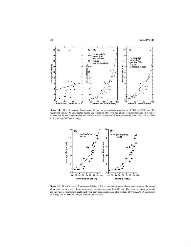
Figure 14. Plot of average fluorescence lifetime at an emission wavelength of 500 nm (380 nm LED
excitation) versus (A) uncorrected alkane concentration, (B) corrected alkane concentration and (C) sum of
uncorrected alkane concentration and column losses. Reproduced with permission from Ref [22], © 2004,
Society for applied Spectroscopy.
20 30 40 50 60 70 80 90 100
0
2
4
6
8
10
(A)
y=a*exp(b*x),
r=0.88
average lifetime [ns]
corrected alkane [%]
20 30 40 50 60 70 80 90 100
0
2
4
6
8
10
(B)
y=a*exp(b*x),
r=0.88
average lifetime [ns]
alkane & loss[%]
Figure 15. Plot of average fluorescence lifetime (τ ) versus: A) corrected alkane concentration; B) sum of
alkane concentration and column losses at the emission wavelength of 540 nm. The best exponential growth fit
and the value of correlation coefficient r for each concentration are also plotted. Reproduced with permission
from Ref [32], © 2004, Society for applied Spectroscopy.
A. G. RYDER
0
2
4
6
8
10
12
14
16
18
20
40
60
80
100
y = a(exp(bx)),
std-err:2.62
max dev:6.60,
r
2
=0.65
a=0.197, b=0.0456
(B)
Alkane conc. (%w/w, corr.)
Average lifetime, ns.
0
2
4
6
8
10
12
14
16
18
40
60
80
100
(C)
y = a(exp(bx)),
std-err:2.47
max dev:7.16,
r
2
=0.69
a=0.0356, b=0.0603
Alkane & Losses % (w/w )
Average lifetime, ns
0
2
4
6
8
10
12
14
16
18
10
30
50
70
(A)
Alkane conc. (%w/w, uncorr.)
Average lifetime (ns)
Figure 14. Plot of average fluorescence lifetime at an emission wavelength of 500 nm (380 nm LED
excitation) versus (A) uncorrected alkane concentration, (B) corrected alkane concentration and (C) sum of
uncorrected alkane concentration and column losses. Reproduced with permission from Ref [22], © 2004,
Society for applied Spectroscopy.
20 30 40 50 60 70 80 90 100
0
2
4
6
8
10
(A)
y=a*exp(b*x),
r=0.88
average lifetime [ns]
corrected alkane [%]
20 30 40 50 60 70 80 90 100
0
2
4
6
8
10
(B)
y=a*exp(b*x),
r=0.88
average lifetime [ns]
alkane & loss[%]
Figure 15. Plot of average fluorescence lifetime (τ ) versus: A) corrected alkane concentration; B) sum of
alkane concentration and column losses at the emission wavelength of 540 nm. The best exponential growth fit
and the value of correlation coefficient r for each concentration are also plotted. Reproduced with permission
from Ref [32], © 2004, Society for applied Spectroscopy.