

7.5. TRANSIENT WAVE GENERATION
391
as
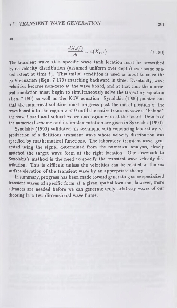
dXo(t)
dt
=ü(Xo,t)
(7.180)
The transient wave at a specific wave tank location must be prescribed
by its velocity distribution (assumed uniform over depth) over some spatial extent at time t0. This initial condition is used as input to solve the
KdV equation (Eqn. 7.179) marching backward in time. Eventually, wave
velocities become non-zero at the wave board, and at that time the numerical simulation must begin to simultaneously solve the trajectory equation
(Eqn. 7.180) as well as the KdV equation. Synolakis (1990) pointed out
that the numerical solution must progress past the initial position of the
wave board into the region x < 0 until the entire transient wave is “behind”
the wave board and velocities are once again zero at the board. Details of
the numerical scheme and its implementation are given in Synolakis (1990).
Synolakis (1990) validated his technique with convincing laboratory reproduction of a fictitious transient wave whose velocity distribution was
specified by mathematical functions. The laboratory transient wave, generated using the signal determined from the numerical analysis, closely
matched the target wave form at the right location. One drawback to
Synolakis’s method is the need to specify the transient wave velocity distribution. This is difficult unless the velocities can be related to the sea
surface elevation of the transient wave by an appropriate theory.
In summary, progress has been made toward generating some specialized
transient waves of specific form at a given spatial location; however, more
advances are needed before we can generate truly arbitrary waves of our
choosing in a two-dimensional wave flume.
391
as
dXo(t)
dt
=ü(Xo,t)
(7.180)
The transient wave at a specific wave tank location must be prescribed
by its velocity distribution (assumed uniform over depth) over some spatial extent at time t0. This initial condition is used as input to solve the
KdV equation (Eqn. 7.179) marching backward in time. Eventually, wave
velocities become non-zero at the wave board, and at that time the numerical simulation must begin to simultaneously solve the trajectory equation
(Eqn. 7.180) as well as the KdV equation. Synolakis (1990) pointed out
that the numerical solution must progress past the initial position of the
wave board into the region x < 0 until the entire transient wave is “behind”
the wave board and velocities are once again zero at the board. Details of
the numerical scheme and its implementation are given in Synolakis (1990).
Synolakis (1990) validated his technique with convincing laboratory reproduction of a fictitious transient wave whose velocity distribution was
specified by mathematical functions. The laboratory transient wave, generated using the signal determined from the numerical analysis, closely
matched the target wave form at the right location. One drawback to
Synolakis’s method is the need to specify the transient wave velocity distribution. This is difficult unless the velocities can be related to the sea
surface elevation of the transient wave by an appropriate theory.
In summary, progress has been made toward generating some specialized
transient waves of specific form at a given spatial location; however, more
advances are needed before we can generate truly arbitrary waves of our
choosing in a two-dimensional wave flume.