7.3. FIRST-ORDER WAVE GENERATION
341
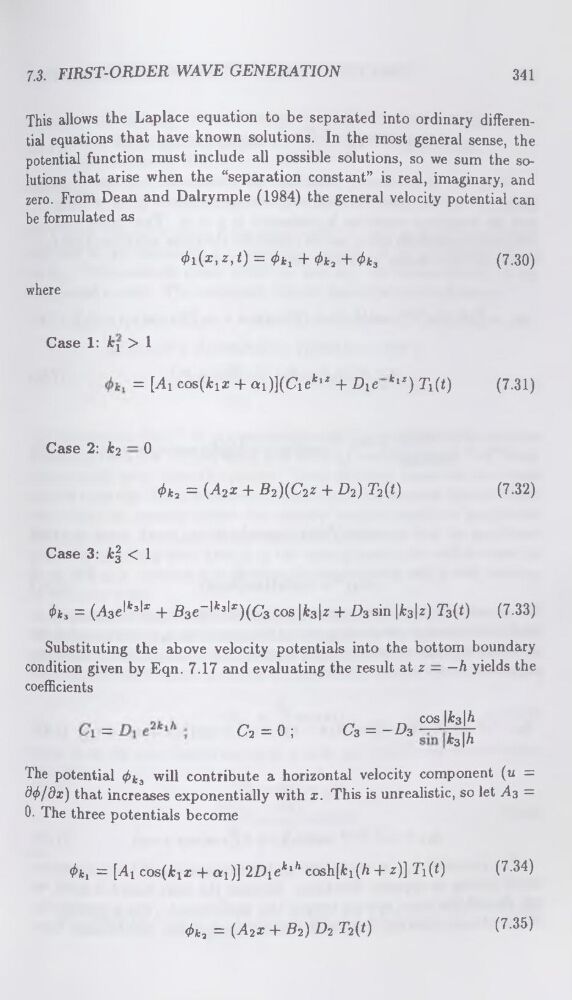
This allows the Laplace equation to be separated into ordinary differential equations that have known solutions. In the most general sense, the
potential function must include all possible solutions, so we sum the solutions that arise when the “separation constant” is real, imaginary, and
zero. From Dean and Dalrymple (1984) the general velocity potential can
be formulated as
<^i(x,z,t) = kl + ki + (7.30)
where
Case 1: fcj > 1
= [Al cos(fciz + ai)](C'iefc12 + Dxe k'z)Tx(t)
(7.31)
Case 2: k2 — 0
<^2 = (A2x 4- B2)(C22 + D2) T2(/)
(7.32)
Case 3: fcf < 1
h, = CA3el‘’l' + B3e’|l3k)(C3 cos |t3|z + D3 sin |t3|3) T3(i)
(7.33)
Substituting the above velocity potentials into the bottom boundary
condition given by Eqn. 7.17 and evaluating the result at z — —h yields the
coefficients
„ cos IXrsITi
=
c, = o;
c3 = -B3-J^
The potential (ty/dx) that increases exponentially with x. This is unrealistic, so let A3 =
0. The three potentials become
(/>kl = [Ai cos(fciz + aj] 2D1e * 1/l cosh[fci(/i + z)] Tx(t)
(7-34)
k2 = (A2x + B2) D2 T2(t)
(7.35)