

7.3. FIRST-ORDER WAVE GENERATION
339
which can be written in Cartesian coordinates for the particular wave board
configuration shown in Figure 7.1 as
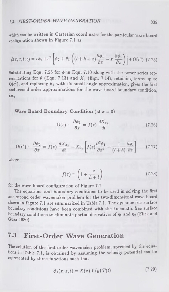
0(i, z,t", c) — c0i 4-e2 02 +
<90i
Y
dx
X dz) + O(c3) (7.25)
Substituting Eqn. 7.25 for 0 in Eqn. 7.10 along with the power series representations for 9 (Eqn. 7.13) and Xo (Eqn. 7.14), retaining terms up to
0(c2), and replacing 9r with its small angle approximation, gives the first
and second order approximations for the wave board boundary condition,
i.e.,
Wave Board Boundary Condition (at x = 0)
0(f): ^ = /(z)^r
(726)
2\
^02
\ d.X o
f(\& 01
1
<90i
.
.
o(<).
<7-27>
where
/(*) =
(7.28)
for the wave board configuration of Figure 7.1.
The equations and boundary conditions to be used in solving the first
and second order wavemaker problem for the two-dimensional wave board
shown in Figure 7.1 are summarized in Table 7.1. The dynamic free surface
boundary conditions have been combined with the kinematic free surface
boundary conditions to eliminate partial derivatives of 771 and 772 (Flick and
Guza 1980).
7.3 First-Order Wave Generation
The solution of the first-order wavemaker problem, specified by the equations in Table 7.1, is obtained by assuming the velocity potential can be
represented by three functions such that
^(x,z,t) = X(x)Y(y) T(t)
(7.29)
339
which can be written in Cartesian coordinates for the particular wave board
configuration shown in Figure 7.1 as
0(i, z,t", c) — c0i 4-e2 02 +
<90i
Y
dx
X dz) + O(c3) (7.25)
Substituting Eqn. 7.25 for 0 in Eqn. 7.10 along with the power series representations for 9 (Eqn. 7.13) and Xo (Eqn. 7.14), retaining terms up to
0(c2), and replacing 9r with its small angle approximation, gives the first
and second order approximations for the wave board boundary condition,
i.e.,
Wave Board Boundary Condition (at x = 0)
0(f): ^ = /(z)^r
(726)
2\
^02
\ d.X o
f(\& 01
1
<90i
.
.
o(<).
<7-27>
where
/(*) =
(7.28)
for the wave board configuration of Figure 7.1.
The equations and boundary conditions to be used in solving the first
and second order wavemaker problem for the two-dimensional wave board
shown in Figure 7.1 are summarized in Table 7.1. The dynamic free surface
boundary conditions have been combined with the kinematic free surface
boundary conditions to eliminate partial derivatives of 771 and 772 (Flick and
Guza 1980).
7.3 First-Order Wave Generation
The solution of the first-order wavemaker problem, specified by the equations in Table 7.1, is obtained by assuming the velocity potential can be
represented by three functions such that
^(x,z,t) = X(x)Y(y) T(t)
(7.29)