

10. Numerical Modelling
333
has proven to converge several orders of magnitude faster than any direct
schemes. The algorithm is as given below.
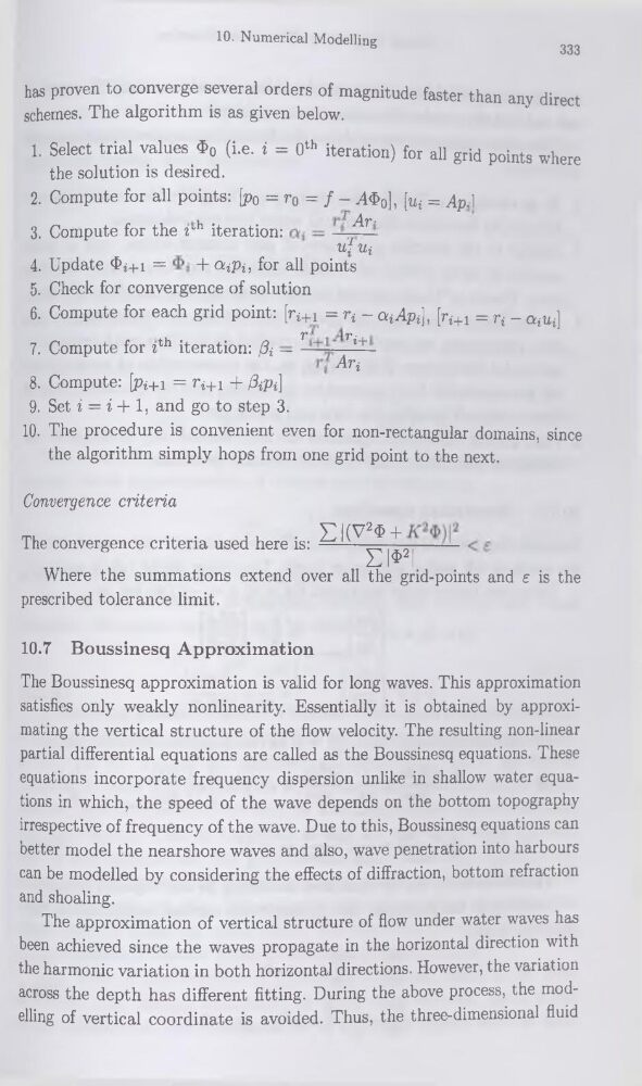
1. Select trial values £0 (i.e. i = 0th itération) for ail grid points where
the solution is desired.
2. Compute for ail points: [p0 = r0 = f - A£o], [u; = ApA
,
Ar '
3. Compute for the rh itération:
ujui
4. Update <Êq+i = + o^Pi, for ail points
5. Check for convergence of solution
6. Compute for each grid point: [ri+1 = n - aiApi], [ri+1 = n - aiUi]
y*
T* '
7. Compute for zth itération: fa —
—!±_
Ati
8. Compute: [pi+i = ri+1 + fe]
9. Set i = i + 1, and go to step 3.
10. The procedure is convenient even for non-rectangular domains, since
the algorithm simply hops from one grid point to the next.
Convergence criteria
The convergence criteria used here is:
E |(v2$ +
ER
Where the summations extend over ail the grid-points and e is the
prescribed tolérance limit.
10.7 Boussinesq Approximation
The Boussinesq approximation is valid for long waves. This approximation
satisfies only weakly nonlinearity. Essentially it is obtained by approximating the vertical structure of the flow velocity. The resulting non-linear
partial differential équations are called as the Boussinesq équations. These
équations incorporate frequency dispersion unlike in shallow water équations in which, the speed of the wave dépends on the bottom topography
irrespective of frequency of the wave. Due to this, Boussinesq équations can
better model the nearshore waves and also, wave pénétration into harbours
can be modelled by considering the effects of diffraction, bottom refraction
and shoaling.
The approximation of vertical structure of flow under water waves has
been achieved since the waves propagate in the horizontal direction with
the harmonie variation in both horizontal directions. However, the variation
across the depth has different fitting. During the above process, the modelling of vertical coordinate is avoided. Thus, the three-dimensional fluid
333
has proven to converge several orders of magnitude faster than any direct
schemes. The algorithm is as given below.
1. Select trial values £0 (i.e. i = 0th itération) for ail grid points where
the solution is desired.
2. Compute for ail points: [p0 = r0 = f - A£o], [u; = ApA
,
Ar '
3. Compute for the rh itération:
ujui
4. Update <Êq+i = + o^Pi, for ail points
5. Check for convergence of solution
6. Compute for each grid point: [ri+1 = n - aiApi], [ri+1 = n - aiUi]
y*
T* '
7. Compute for zth itération: fa —
—!±_
Ati
8. Compute: [pi+i = ri+1 + fe]
9. Set i = i + 1, and go to step 3.
10. The procedure is convenient even for non-rectangular domains, since
the algorithm simply hops from one grid point to the next.
Convergence criteria
The convergence criteria used here is:
E |(v2$ +
ER
Where the summations extend over ail the grid-points and e is the
prescribed tolérance limit.
10.7 Boussinesq Approximation
The Boussinesq approximation is valid for long waves. This approximation
satisfies only weakly nonlinearity. Essentially it is obtained by approximating the vertical structure of the flow velocity. The resulting non-linear
partial differential équations are called as the Boussinesq équations. These
équations incorporate frequency dispersion unlike in shallow water équations in which, the speed of the wave dépends on the bottom topography
irrespective of frequency of the wave. Due to this, Boussinesq équations can
better model the nearshore waves and also, wave pénétration into harbours
can be modelled by considering the effects of diffraction, bottom refraction
and shoaling.
The approximation of vertical structure of flow under water waves has
been achieved since the waves propagate in the horizontal direction with
the harmonie variation in both horizontal directions. However, the variation
across the depth has different fitting. During the above process, the modelling of vertical coordinate is avoided. Thus, the three-dimensional fluid