

10. Numerical Modelling
331
Finite différence method
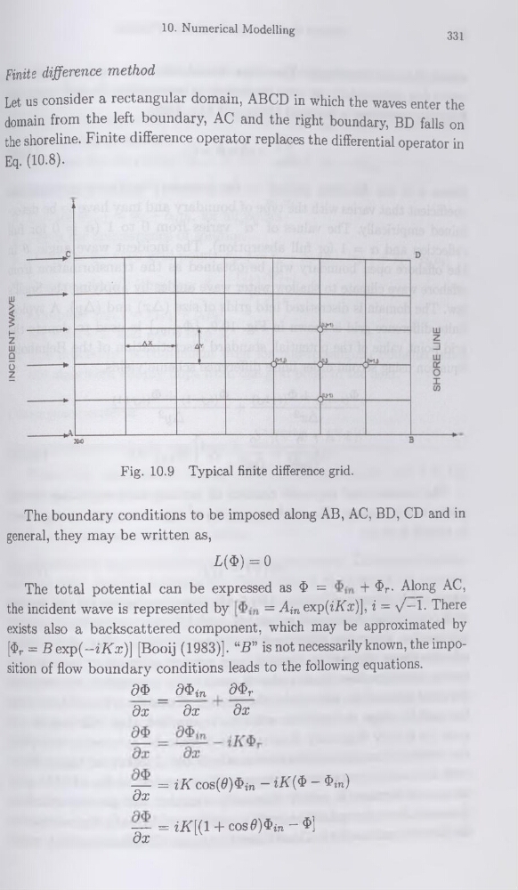
Let us consider a rectangular domain) ABCD in which the waves enter the
domain from the left boundary, AC and the right boundary, BD falls on
the shoreline. Finite différence operator replaces the differential operator in
Eq. (10.8).
Fig. 10.9 Typical finite différence grid.
The boundary conditions to be imposed along AB, AC, BD, CD and in
general, they may be written as,
L(£) =0
The total potential can be expressed as $ =
+ $r- Along AC,
the incident wave is represented by
= Ajnexp(iÀ’x)], i = x/-ï. There
exists also a backscattered component, which may be approximated by
[$r = Bexp(-zATc)] [Booij (1983)]. “B” is not necessarily known, the imposition of flow boundary conditions leads to the following équations.
< 9$ _ d$in
d$r
dx
dx
dx
— — = iK COs(0)$in - îA($ - $in)
dx
— = iK[(l +cos 0)$in-$]
dx
331
Finite différence method
Let us consider a rectangular domain) ABCD in which the waves enter the
domain from the left boundary, AC and the right boundary, BD falls on
the shoreline. Finite différence operator replaces the differential operator in
Eq. (10.8).
Fig. 10.9 Typical finite différence grid.
The boundary conditions to be imposed along AB, AC, BD, CD and in
general, they may be written as,
L(£) =0
The total potential can be expressed as $ =
+ $r- Along AC,
the incident wave is represented by
= Ajnexp(iÀ’x)], i = x/-ï. There
exists also a backscattered component, which may be approximated by
[$r = Bexp(-zATc)] [Booij (1983)]. “B” is not necessarily known, the imposition of flow boundary conditions leads to the following équations.
< 9$ _ d$in
d$r
dx
dx
dx
— — = iK COs(0)$in - îA($ - $in)
dx
— = iK[(l +cos 0)$in-$]
dx